-
Title
-
Occurrence and distribution of Dinophysis Spp. in Budd Inlet, Washington during a seasonal cycle from winter to fall of 2019: Possible causative environmental factors
-
Date
-
2019
-
Creator
-
Estrada-Packer, Naomi
-
Identifier
-
Thesis_MES_2019_Estrada-PackerN
-
extracted text
-
OCCURRENCE AND DISTRIBUTION OF DINOPHYSIS SPP. IN BUDD INLET,
WASHINGTON DURING A SEASONAL CYCLE FROM WINTER TO FALL
OF 2019: POSSIBLE CAUSATIVE ENVIRONMENTAL FACTORS
by
Naomi Estrada-Packer
A Thesis
Submitted in partial fulfillment
of the requirements for the degree
Master of Environmental Studies
The Evergreen State College
December 2019
��©2019 by Naomi Estrada-Packer. All rights reserved.
��This Thesis for the Master of Environmental Studies Degree
by
Naomi Estrada-Packer
has been approved for
The Evergreen State College
by
________________________
Gerardo Chin-Leo, Ph. D.
Member of the Faculty
________________________
Date
��ABSTRACT
Occurrence and Distribution of Dinophysis spp. in Budd inlet, Washington during a
seasonal cycle from Winter to Fall of 2019: Possible Causative Environmental Factors
Naomi Estrada-Packer
Harmful algal blooms (HABs) are a major environmental problem. This study focused on
Dinophysis, a HAB genus of marine dinoflagellates capable of producing phycotoxins
responsible for diarrhetic shellfish poisoning (DSP) events. During a 10-month period
(Jan-Oct 2019), I monitored phytoplankton species composition and biomass, and
determined cell densities of various Dinophysis species (D. norvegica, D. acuminata, D.
fortii, D. rotundata, D. parva, and D. odiosa) at 2 stations with different oceanographic
conditions in Budd Inlet, one at the head and other at the mouth of the estuary. A
sampling method was developed to detect Dinophysis at low cell concentrations (> 2
cells/L). Samples were collected weekly (spring to summer) to monthly (fall and winter).
To determine the environmental factors explaining Dinophysis abundance, water quality
and physicochemical parameters were measured and data on meteorological conditions
were examined. In addition, DSP toxin data from Washington Department of Health was
obtained to determine if DSP toxin levels coincided with Dinophysis abundance. There
were significant changes in phytoplankton species composition over space and time.
Diatoms dominated in winter and dinoflagellates dominated in spring /summer.
Dinoflagellates were more abundant at the head of the estuary and diatoms at the mouth.
Dinophysis species were found in all but one sampling time with D. norvegica being the
most common species. The largest D. norvegica abundance occurred at both stations
during summer reaching densities of 23,857 cells/L at the estuary head and 3,590 cells/L
at the mouth. While the cell densities at the head were greater than the mouth, blooms
coincided over time suggesting widespread meteorological conditions may explain the
timing of blooms with local differences in stratification and nutrients determining
abundance. Chemical and physical parameters at both stations were significantly different
(p<0.05). At the head of the estuary, river discharge, surface water temperature, nitrate
and phosphate and nutrient ratios were strongly related to Dinophysis abundance
suggesting that Dinophysis benefits from stratified conditions and proximity to the river
nutrient source. DSP toxin levels were not significantly related to Dinophysis abundance.
Toxicity of Dinophysis may be species-specific where individual species could be more
toxic than others. The dominance of D. norvegica, a species with relatively low toxicity
may explain this apparent discrepancy.
��TABLE OF CONTENTS
List of Figures...............................................................................................................xi
List of Tables.............................................................................................................xv
List of Appendices…………………………………………………………………xvi
Acknowledgements..................................................................................................xvii
CHAPTER 1: INTRODUCTION
1.1: What are Harmful Algal Blooms (HABs)……………………………………..…1
1.2: Significance………………..……………………………………………………..1
1.3: Humans as Cause and Victims of HABs…………………………………………2
1.4: Concerns of Dinophysis in Washington State……………………………..……..3
1.5: Local Research Efforts………………………………………………….………..4
1.6: My Research Efforts and Contribution…………………………………………..5
1.7: Research Objectives: Question-Hypothesis-Approach…………………….…….6
CHAPTER 2: LITERATURE REVIEW
2.1: Overview of Biology & Ecology of the genus Dinophysis……………….……...7
2.2: Diarrhetic Shellfish Poisoning (DSP)…………………………..……………….11
2.2.1: History and Global Distribution of DSP events…………………....…12
2.2.2: DSP Events in the Puget Sound…………………..…………………..14
2.3: Trophic Dynamics and Diarrhetic Shellfish Toxins in Puget Sound…………...16
2.4: Ecophysiology of Dinophysis in Estuarine-Coastal Ecosystems…………..…...19
2.4.1: Eutrophication and Toxic Dinophysis…………………………...……20
2.4.2: Theory of Ecological Roles of DSTs………………………..………..22
2.5: Ecophysiological Response of Dinophysis ……………………………………..25
2.5.1: Response to Nutrients and Eutrophic Conditions……………..……...27
2.5.2: Response to Hydrological and Other Environmental Parameters…….29
2.6: Toxic Dinophysis in Budd Inlet……………………………………………...….32
CHAPTER 3: MATERIALS AND METHODS
3.1: Study Area and Monitoring Stations…….............................................................34
3.2: Research Design: Field Sample Collection and Lab Processing...........................36
3.3: Dinophysis, DSTs, and Environmental Analyses………………………………..37
3.3.1: Dinophysis Abundance and Species Composition…………………….37
3.3.2: Measurements of Environmental Parameters………………………….38
3.4: Statistical Analyses………………………………………………………………39
CHAPTER 4: RESULTS
4.1: Phytoplankton Species Composition......................................................................41
4.2: Spatiotemporal Differences ...................................................................................42
4.3: Dinophysis Species Diversity and Abundance…………………………………...45
4.4: Spatiotemporal Distribution of Dinophysis Species……………………………...46
4.5: Influence of Environmental Conditions on the Distribution of Dinophysis……...48
4.6: Shellfish Toxicity………………............................................................................82
ix
�CHAPTER 5: DISCUSSION
5.1: Overview of Research Questions & Hypotheses.......................................................85
5.2: Phytoplankton Species Composition and Primary Productivity................................86
5.3: Spatiotemporal Distribution of Dinophysis spp. .......................................................87
5.4 Dinophysis Abundances and Environmental Factors..................................................88
5.5: Suggestions for Future Research................................................................................94
x
�LIST OF FIGURES
Figure 1: Chemical structures of okadaic acid and its congeners of dinophysistoxin-1
and dinophysistoxin-2 (DTX-1 and DTX-2)……………………………………….....9
Figure 2 (adapted from Prego-Faraldo et al., 2013): The transfer of OA and DTXs
through the food chain.………………………………………………………….…...17
Figure 3: Two monitoring stations within Budd Inlet, South Puget Sound, WA…...35
Figure 4: Time series of biomass (chlorophyll-a) levels throughout the annual seasonal cycle
at the estuary head (NPL) in Budd Inlet……………………………………………..43
Figure 5: Time series of biomass (chlorophyll-a) levels throughout the annual seasonal cycle
at the mouth of the estuary (BHM) in Budd Inlet………………………………….. 44
Figure 6: Dinophysis abundance over the seasonal cycle from winter to fall of 2019 at the
estuary head (NPL) and mouth (BHM) in Budd Inlet, WA. ………………………. 48
Figure 7: Time series of phosphate levels over the seasonal cycle of winter to fall of 2019 at
the estuary head (BHM) in Budd Inlet………………………………………………52
Figure 8: Time series of phosphate levels over the seasonal cycle of spring to fall of 2019 at
the estuary mouth (NPL) in Budd Inlet.……………………………………………..52
Figure 9: Time series of Dinophysis abundance versus phosphate levels at the estuary head
(NPL) in Budd Inlet. .……………………………….…………………………..……53
Figure 10: Time series of Dinophysis abundance versus phosphate levels at the estuary
mouth (BHM) in Budd Inlet. .………………………………………………………...53
Figure 11: Time series of phosphate levels over the seasonal cycle of spring to fall of 2019 at
the estuary head (NPL) in Budd Inlet…………………………………………………54
Figure 12: Time series of Dinophysis abundance versus nitrate levels at the estuary head
(NPL) in Budd Inlet………………………………………………………….……..….55
Figure 13: Time series of phosphate levels over the seasonal cycle of spring to fall of
2019 at the estuary head (NPL) in Budd Inlet…………………………………………55
Figure 14: Time series of Dinophysis abundance versus nitrate levels at the estuary mouth
(BHM) in Budd Inlet.………………………………………………………………….56
Figure 15: Time series of nutrient ratios of dissolved silica to dissolved inorganic phosphate
(DSI:DIP) over the seasonal cycle of spring to fall of 2019 at the estuary head (NPL) in Budd
Inlet………………………………………………………..…………………………..58
xi
�Figure 16: Time series of nutrient ratios of dissolved silica to dissolved inorganic phosphate
(DSI:DIP) over the seasonal cycle of spring to fall of 2019 at the estuary mouth (BHM) in
Budd Inlet.……………………………………………………………………………………58
Figure 17: Time series of Dinophysis abundance versus nutrient ratios of dissolved silica to
dissolved inorganic phosphate (DSI:DIP) at the estuary head (NPL) in Budd Inlet………...59
Figure 18: Time series of Dinophysis abundance versus nutrient ratios of dissolved silica to
dissolved inorganic phosphate (DSI:DIP) at the estuary mouth (BHM) in Budd Inlet……...59
Figure 19: Time series of nutrient ratios of dissolved inorganic nitrogen to dissolved
inorganic phosphate (DIN:DIP) over the seasonal cycle of spring to fall of 2019 at the estuary
head (NPL) in Budd Inlet…………….……………………………………………………....60
Figure 20: Time series of Dinophysis abundance versus nutrient ratios of dissolved inorganic
nitrogen to dissolved inorganic phosphate (DIN:DIP) at the estuary head (NPL) in Budd
Inlet……………………………………………………………………………………...…...61
Figure 21: Time series of nutrient ratios of dissolved inorganic nitrogen to dissolved
inorganic phosphate (DIN:DIP) over the seasonal cycle of spring to fall of 2019 at the estuary
mouth (BHM) in Budd Inlet………………………………………………………………….61
Figure 22: Time series of Dinophysis abundance versus ammonium levels at the estuary
mouth (BHM) in Budd Inlet………………………………………………………………….62
Figure 23: Time series of ammonium levels over the seasonal cycle of spring to fall of 2019
at the estuary head (BNPL) in Budd Inlet. ………………………………..…………………63
Figure 24: Time series of Dinophysis abundance versus ammonium levels at the estuary head
(NPL) in Budd Inlet. ………………………………...………………………………….…...64
Figure 25: Time series of ammonium levels over the seasonal cycle of spring to fall of 2019
at the estuary mouth (BHM) in Budd Inlet. …………………………………..………...…...64
Figure 26: Time series of Dinophysis abundance versus ammonium levels at the estuary
mouth (BHM) in Budd Inlet. ………………………………..…………………………….....65
Figure 27: Time series of dissolved oxygen levels over the seasonal cycle of spring to fall of
2019 at the estuary mouth (BHM) in Budd Inlet. ………………………………….………..67
Figure 28: Time series of Dinophysis abundance versus dissolved oxygen levels at the
estuary head (NPL) in Budd Inlet. ……………………………………...…………………...68
Figure 29: Time series of dissolved oxygen levels over the seasonal cycle of spring to fall of
2019 at the estuary mouth (BHM) in Budd Inlet………………………………………….....68
xii
�Figure 30: Time series of Dinophysis abundance versus dissolved oxygen levels at the
estuary mouth (BHM) in Budd Inlet. …………………………………………………….….69
Figure 31: Time series of air and surface water temperatures over the seasonal cycle of
spring to fall of 2019 at the estuary head (NPL) in Budd Inlet. ……………………………70
Figure 32: Time series of air and surface water temperatures (1m depth) over the seasonal
cycle of spring to fall of 2019 at the estuary mouth (BHM) in Budd Inlet. …………………71
Figure 33: Time series of Dinophysis abundance versus surface water temperatures (1m
depth) at the estuary head (NPL) in Budd Inlet. ………………………………………….....71
Figure 34: Time series of Dinophysis abundance versus surface water temperatures (1m
depth) at the estuary mouth (BHM) in Budd Inlet. …………….……………………………72
Figure 35: Time series of the Deschutes River discharge into Budd Inlet during the seasonal
cycle of winter to fall of 2019. …………………….………………………………………...73
Figure 36: Time series of Dinophysis abundance versus river discharge at the estuary head
(NPL) in Budd Inlet. ……………………………………………………….……………..…73
Figure 37: Time series of Dinophysis abundance versus river discharge at the estuary mouth
(BHM) in Budd Inlet. ……………………………………………………………..………....74
Figure 38: Time series of the wind speed and direction in Budd Inlet during the seasonal
cycle of winter to fall of 2019. ……………………………………………………………....75
Figure 39: Time series of Dinophysis abundance versus wind speed at the estuary head
(NPL) in Budd Inlet……………………………………………………………….…………75
Figure 40: Time series of Dinophysis abundance versus wind speed at the estuary mouth
(BHM) in Budd Inlet…………………………………………………………………............76
Figure 41: Time series of solar radiation in Budd Inlet during the seasonal cycle of winter to
fall of 2019.…………………………………………………………………………….….....77
Figure 42: Time series of Dinophysis abundance versus solar radiation at the estuary head
(NPL) in Budd Inlet…………………………………………………………………….........77
Figure 43: Time series of Dinophysis abundance versus solar radiation at the estuary mouth
(BHM) in Budd Inlet………………………………………………………………………....78
Figure 44: Time series of solar radiation in Budd Inlet during the seasonal cycle of winter to
fall in 2019………………………………………….………………………..………………79
Figure 45: Time series of Dinophysis abundance versus average rainfall at the estuary head
(NPL) in Budd Inlet……...………………………………………………………………..…80
xiii
�Figure 46: Time series of Dinophysis abundance versus average rainfall at the estuary mouth
(BHM) in Budd Inlet. ……………………………………………………………………..…80
Figure 47: Time series of average rainfall and ammonium levels at the estuary head (NPL)
during the seasonal cycle of winter to fall in 2019…………………………………………..81
Figure 48: Time series of average rainfall and ammonium levels at the estuary mouth (BHM)
during the seasonal cycle of winter to fall in 2019…………………………………………..81
Figure 49: Time series of Dinophysis abundance versus the total DSP toxin levels at the
estuary head (NPL) during the seasonal cycle of winter to fall in 2019…………………..…83
Figure 50: Time series of Dinophysis abundance versus the total DSP toxin levels at the
estuary mouth (BHM) during the seasonal cycle of winter to fall in 2019…………………..84
xiv
�LIST OF TABLES
Table 1: Differences in environmental parameters between the estuary head and estuary
mouth…………………………………………………………………………………......…..43
Table 2: Regression analysis between biomass and environmental parameters at the estuary
head (NPL) and mouth (BHM) in Budd Inlet…………………………………………….….45
Table 3: Independent means t-test statistical analysis of Dinophysis abundance related to
biomass (chlorophyll-a)……………………………. ……………………………………….49
Table 4: Simple linear regression analysis of Dinophysis abundance related to nutrients
(nitrate, ammonium, silicate, and phosphorous) at the estuary mouth (NPL) and head (BHM)
in Budd Inlet………………………………………………...………………………..………51
Table 5: Simple linear regression analysis of Dinophysis abundance related to nutrients ratios
at the estuary mouth (NPL) and head (BHM) in Budd Inlet……………………………...….57
Table 6: Simple linear regression analysis of Dinophysis abundance related to meteorological
conditions at the estuary mouth (NPL) and head (BHM) in Budd Inlet………………..……66
Table 7: Simple linear regression analysis of Dinophysis abundance related to water quality
parameters at the estuary mouth (NPL) and head (BHM) in Budd Inlet…………….……....66
Table 8: Regression analysis between Dinophysis abundance versus DSP toxins at the
estuary head and mouth in Budd Inlet)…………………………….………………………...84
xv
�LIST OF APPENDICES
Appendix A: Species Composition Supporting Data………………………………............119
Appendix B: Dinoflagellate Scanning Electron Project……………………………………138
xvi
�Acknowledgements
This has been a tremendous educational journey about growing as a person, student, and
a scientist. I am honored to have learned and delved in deep into this particular subject
involving our precious waters and the living organisms that need our attention and utmost
care. If it were not for support of my advisor Gerardo Chin-Leo, Vera Trainer and Brian
Bill from the SoundToxins team, Jerry Borchert from WDOH, Nick (my husband), my
family, friends and ancestors, I would not come this far without you all. I thank you all
from the depths of my soul for all of your guidance throughout this educational
experience. All of you have inspired me to keep striving and moving forward no matter
what obstacles lie ahead and continue to be a steward to our Earth and its waters.
Thank you all so much!
xvii
��CHAPTER 1: INTRODUCTION
1.1: What are HABs?
Harmful Algal Blooms (HAB) are a global phenomenon impacting most marine
ecosystems particularly in coastal and estuarine regions (Lelong et al., 2012). Highdensity blooms of phytoplankton—microscopic algae—produce biotoxins, also known as
phycotoxins, affecting aquatic life and ecosystems along with human health (Anderson et
al., 2012). There is a general scientific consensus that the number of toxic blooms,
resulting economic losses of shellfish industries, disruption of subsistence practices, and
the number of toxins and toxic species reported have all increased over the last few
decades (2012). In Washington, HAB’s have only been recently detected along the coast
and within Puget Sound. The quality of marine waters has become a particularly
important issue due to a large populace using aquatic resources involving shellfish
industries and tribal subsistence. There are various state and government organizations
extending great effort toward studying HABs. These agencies include: SoundToxins—
National Ocean and Atmospheric Administration (NOAA), Washington Department of
Health (WDOH), Olympic Region Harmful Algal Blooms (ORHAB), and Puget Sound
Marine Monitoring.
1.2: Significance
HABs toxins are concentrated by bivalves (e.g. blue mussels and other shellfish),
which filter feeders consume the toxic phytoplankton. Humans are affected by the toxins
when they consume the contaminated shellfish. Exposure to toxins over the USDA action
levels can cause health illnesses related to Diarrheic Shellfish Poisoning (DSP), Amnesic
Shellfish Poisoning (ASP), Paralytic Shellfish Poisoning (PSP), and Neurotoxin Shellfish
1
�Poisoning (NSP) (Grattan et al. 2016). Most HAB related illnesses have similar
symptoms to gastrointestinal and neurological problems (Grattan et al., 2016). The
impacts of HABs not only affect humans but can also affect wildlife that consume
contaminated phytoplankton or shellfish causing similar yet more severe illness which
can lead to death (Anderson, Cembella, & Hallegraeff, 2012).
1.3: Humans as Cause and Victims of HABs
HAB occurrence is associated with a complex set of physical, chemical,
biological, hydrological, and meteorological conditions making it difficult to determine
the causative factors. However, severe HAB events in coastal and estuarine areas have
been related to anthropogenic activities (Lelong et al., 2012; Lehmann & Gobler, 2015).
Extensive HAB research has been conducted over the past decades, and several
anthropogenic mechanisms stimulating toxic bloom events have been identified. These
include: 1) natural dispersal of species by currents and storms; 2) dispersal through
human activities (such as ballast water discharge and shellfish translocation); 3) increased
aquaculture operations in coastal waters; 4) increased anthropogenic eutrophication and
climate change (Anderson et al., 2012; Lelong et al., 2012). HABs pose a major threat to
human health. Therefore, it is essential to predict the occurrence of toxic blooms, their
toxin production, and toxicity per cell in order to effectively continue to develop
proactive management of coastal resources and minimize humans and public health risks
(Anderson et al., 2012).
Anthropogenic inputs of excess nutrients of nitrogen, phosphorous, and
ammonium have all been determined to alter the nutrient ratios leading to negatively
affecting phytoplankton species composition and facilitating the onset and development
2
�of toxic blooms (Davidson et al., 2016; Flynn, 2010; Pan, Bates, & Cembella, 1998). Due
to the scarcity of particular nutrients (i.e. silica) and nutrient loading of nitrogen and
phosphorous, phytoplankton have evolved to adapt to their surrounding waters. With
these anthropogenic environmental pressures, as phytoplankton—both dinoflagellates and
diatoms—evolved they have developed adaptations to outcompete other species for
nutrients and defenses against other phytoplankton predators and grazers (Rossini, 2016).
The production of toxins are an example of an adaptation technique to aid in survival of
waters with low water quality and an imbalance of nutrient availability (2016). Toxins
can aid in nutrient and prey acquisition by mixotrophic and autotrophic species of
phytoplankton, and also deter predation from other phytoplankton, zooplankton, bivalves,
and small fish (Smayda, 1997).
1.4: Concerns of Dinophysis in Washington State
Four HAB species have been reported in Puget Sound, Washington for more than
a century, including Dinophysis spp., Pseudo-nitzschia spp., Alexandrium catenella and
Heterosigma akashiwo, although Dinophysis bloom events have more recently been
found (Trainer et al. 2013). The first shellfish closure due to high concentrations of
Diarrheic shellfish toxins, including okadaic acid and dinophysistoxins, occurred in the
Puget Sound in 2011 (Trainer et al. 2013). Due to the increasing frequency of blooms in
the Puget Sound, especially Budd Inlet in South Sound near Olympia, concerns have
been raised about issues regarding the state of water quality and health of marine
organisms within the Puget Sound. Therefore, research scientists and state agencies are
taking great measures to monitor Dinophysis blooms on a frequent basis.
3
�1.5: Local Research Efforts
Due to the potential threats to human and marine organismal health, research
organizations (those mentioned above) are routinely monitoring marine waters
throughout Washington. SoundToxins is a citizen-science monitoring program, managed
by Sea Grant—NOAA located in Puget Sound, WA. SoundToxins plays an integral role in
educating local tribal harvesters, commercial shellfish and fish farmers, and other
partnering state agencies about HABs and the importance of monitoring. SoundToxins
provides a cost-effective, enhanced monitoring program, and emergency response to
notify the possible onset and occurrences of HABs. The local community stakeholders
assist in the decision-making process, thereby enabling the proper harvest the seafood by
ultimately reducing the overall negative impacts to the economy sustained by fisheries in
the Puget Sound, human health, and marine organismal health (SoundToxins, 2018).
WDOH also plays a primary role in minimizing risk and exposure to DSP toxins
caused by Dinophysis spp. occurring throughout the Puget Sound. Sentinel mussels are
continuously monitored by WDOH and sampled for DSP toxins at several sites within
Puget Sound, including Budd Inlet. Collections of mussel tissue are sampled weekly to
bi-weekly for DSP toxins, including okadaic acid, dinophysistoxin-1, and
dinophysistoxin-2. The tissue samples are measured using a Liquid ChromatographyMass Spectrometry (LC-MS) to analyze the concentrations of toxins to detect if the levels
are above the regulatory limit for the public—each toxin has its own regulatory limit
dependent on how fast or slow the toxin is metabolized by the human body. For DSP
toxins, the regulatory limit for safe consumption is 16 micrograms per 100 grams
(Trainer et al. 2013; FDA, 2011).
4
�1.6: My Research Efforts and Contribution
Furthermore, to address the current need for information on the factors that
explain the recurrence and growth of Dinophysis species in Budd Inlet, South Puget
Sound, I decided to pursue a thesis project to understand the environmental conditions
that contribute to Dinophysis blooms, production of Diarrheic Shellfish toxins (DST), and
toxicity profiles and DST levels in mussel tissue. This thesis is contributing to the limited
knowledge of Dinophysis blooms dynamics in relation to environmental conditions at
two locations in Puget Sound with previous Dinophysis presence.
1.7: Research Objectives: Question-Hypothesis-Approach
My two research questions are:
1) What is the spatiotemporal distribution of Dinophysis between the estuary head
(near Deschutes River) and the mouth (near south sound basin) over the seasonal
cycle from winter to fall of 2019 in Budd Inlet?
2) What factors control the abundance of Dinophysis in Budd Inlet, South Puget
Sound, Washington?
I hypothesize the estuary head is environmentally different than the mouth. The
factors of primary activity (biomass), river discharge, stratification, surface water
temperatures, and nutrients (ammonium, nitrate, phosphate) will be the main contributors
to changing environmental conditions between the two stations. These differences may
showcase the particular environmental variables influencing Dinophysis activity in Budd
Inlet.
Several physicochemical factors control Dinophysis abundance during the
seasonal period shifting from spring to summer. These factors include: the rise in surface
5
�water temperatures, an increase in radiation, the limitation of nutrients of phosphorous,
an excess of nitrogen, and an increase in ammonium levels. The Deschutes River
discharge and anthropogenic nutrient inputs of nitrogen and phosphorous from local
wastewater treatments plants and land runoff can greatly influence the composition of
nutrients over the seasonal cycle. Due to the nutrient loading of nitrogen, phosphorous
becomes the limiting factor of dinoflagellates growth during the summer months,
especially when concerning Dinophysis. The alterations of the Redfield ratios of
DSI:DIN and DIN:DIP can shift to support the cellular growth of diatoms during winter
to spring and dinoflagellates from summer to fall. Nutrient ratios are critical to cellular
growth and nutrient uptake, while water quality parameters of low salinity and high
surface water temperatures can also be significant factors positively influencing total
Dinophysis abundance.
To answer this question, this study will investigate phytoplankton species
composition and the dynamics between Dinophysis abundance, environmental conditions,
and toxin profiles (found in mussel tissue) over a 10-month monitoring period (winter to
fall) at two locations within Budd Inlet, Puget Sound—one station at the estuary head
(North Point Landing (NPL)) and the second station at the estuary mouth (Boston Harbor
Marina (BHM)). These sites were chosen because Budd Inlet has been known to have the
highest concentrations of DSP levels recorded in Washington State. In 2016, the DSP
toxin levels were recorded at 250 𝜇g/100g of DSP toxins in blue mussel tissue
(unpublished data, WDOH, Jerry Borchert).
To date, Dinophysis species found in the Puget Sound include: D. acuminata, D.
fortii, D. norvegica, D. acuta, and D. caudata (Trainer et al., 2013). However, their
6
�relative toxicities differ per cell for each species; D. fortii and D. acuminata are two
species that have been known to cause an increase in the levels of okadaic acid and
dinophysistoxins (Trainer et al. 2013). Therefore, this study will identify Dinophysis to
the species level. This will further provide baseline data on the interactions between
Dinophysis presence and particular environmental parameters that potentially influence
intensity, frequency, and toxicity of blooms in the Puget Sound.
Environmental parameters such as air temperature, rainfall, radiation, and wind
patterns will be recorded to understand the seasonality of blooms in relation to associated
environmental parameters. Biologically important water quality parameters such as
surface water temperatures, salinity (stratification), dissolved oxygen, biomass
(chlorophyll-a), and nutrient concentrations of ammonium, phosphorus, nitrogen, and
silica will be measured, along with calculation of nutrient ratios between DIN:DSI:DIP.
The nutrient ratios were computed to determine the changes in nutrient composition.
Variations of these ratios from the Redfield ratios can provide clues on when specific
nutrients are limiting for growth.
I will be analyzing the environmental data to understand if there are qualitative
and statistically significant relationships between Dinophysis abundance and all other
physicochemical, water quality parameter, and DSP toxin levels. Data analysis will be
conducted using time series, regression analysis, and independent t-test analysis to
identify potential environmental mechanisms influencing the spatiotemporal distribution
of Dinophysis species in Budd Inlet, and further understand Dinophysis dynamics to
detect future threats of DSP events in estuarine ecosystems.
7
�CHAPTER 2: LITERATURE REVIEW
2.1: Overview of Biology & Ecology of the genus Dinophysis
The majority of harmful algal blooms (HABs) are caused by toxinproducing dinoflagellates that can be phototrophic, heterotrophic, and
mixotrophic, even though historically HAB species have been thought to be
strictly phototrophs (Anderson et al., 2012). The genus, Dinophysis (“Dino”
meaning “terrible” and “physis” mean “nature”), is characterized as an armored,
mixotrophic, toxin producing dinoflagellate. Dinophysis is a cosmopolitan genus
of dinoflagellates comprised of over 120 taxonomically identified species
(Reguera et al. 2012, 2014; Simoes et al. 2015). Certain species of the Dinophysis
genus have been recently discovered to produce intoxicating phycotoxins known
to have adverse effects on humans and wildlife. To date, only 12 species of
Dinophysis have been identified to synthesize harmful, lipophilic toxins called
okadaic acid (OA) and its congeners of Dinophysistoxin-1 (DTX-1) and
Dinophysistoxin-2 (DTX-2), collectively known as Diarrhetic Shellfish Poisoning
Toxins (DSTs) (Reguera et al., 2014; FAO, 2004) (Figure 1).
8
�Figure 1: Chemical structures of okadaic acid and its congeners of
dinophysistoxin-1 and dinophysistoxin-2 (DTX-1 and DTX-2) (Reguera et al.,
2014).
The toxic species of Dinophysis, include: D. fortii, D. acuminata, D.
norvegica, D. acuta, D. parva, D. caudata, D. infundbulium, D. miles, D.
sacculus, D.ovum, D. tripos, D. rotundata, and D. mitra (Reguera et al., 2014).
Only seven (D. acuminata, D. acuta, D. fortii, D. ovum, D. caudata, D. miles, and
D. sacculus) of these species have been associated with DSP outbreaks worldwide
(Reguera et al., 2012).
Dinophysis (Dinophysaceae) has been identified as the primary organism
to induce harmful algal outbreaks known as Diarrhetic Shellfish Poisoning (DSP)
events (Anderson et al., 2012; Reguera et al., 2012). Although OA, DTX-1, and
DTX-2 are the main contributors to DSP events, Dinophysis species can also coproduce pectenotoxins (PTXs), known to be strictly regulated by the European
Union due to its reported intraperitoneal hepatotoxic effects on mice (Terao et al.,
1986; Reguera et al., 2012). However, PTXs have not been known to cause issues
in other regions of the world, except for Europe where their toxicity has been up
9
�for debate (Reguera & Blanco, 2019). These okadates (OA, DTXs, and PTXs) are
secondary metabolites which are highly stable polyether compounds. Okadates
produced by toxic species of Dinophysis have recently presented increasingly
adverse effects on human health, a condition known as DSP.
Several studies have demonstrated DSTs are biological active compounds
that can promote the onset of various health disorders (Trainer et al., 2013;
Reguera et al., 2014). When DSTs are ingested by humans, various symptoms of
gastrointestinal illness can occur, such as nausea, diarrhea, vomiting, headache,
fever, and severe abdominal pain, with the onset of symptoms occurring within 30
minutes and reducing within a few days (FDA, 2011; Trainer et al. 2013). OA and
dinophysistoxins (DTX-1 and DTX-2) can inhibit protein phosphatases in
mammalian cells by its ability to bind to the receptor site (Cohen et al., 1990).
When consumption of high toxin levels happens, gastrointestinal symptoms occur
due to OA and DTXs triggering increase of phosphorylated proteins, theeby
resulting in hyperphosphorylation of the ion channels in the cells (Cohen et al.,
1990; Cordier et al., 2000; FDA, 2011; Uberhart et al., 2013). Although
gastrointestinal illnesses are most characteristic symptoms of intoxification, OA
and its analogues have been identified to emit tumor-promoting, mutagenic, and
immosuppressive effects, as shown in studies investigating toxicity on mice
(Fujiki & Suganuma, 1999; FAO, 2004. Furthermore, other studies have reported
that chronic exposure to DSTs, specifically OA and DTX-1, promotes
gastrointestinal cancers in humans (Van Egmond et al., 1993; Draisci et al., 1996;
Cordier et al., 2000; Manerio et al., 2008).
10
�2.2: Diarrhetic Shellfish Poisoning
Emergence of DSP occurrences associated with Dinophysis spp. have
increased in frequency and duration on a global scale, progressively posing
various consequences to marine ecosystems, public health, and economic losses to
local shellfish industries (Anderson et al., 2012; Reguera et al., 2012). Due to the
public health consequences, DSTs have been globally recognized and regulated
for the majority of coastal waters with recurring DSP events, however, the United
States does not regulate monitoring for DSTs nationwide. DSTs have been
routinely monitored in Europe and has a regulatory limit of 160 micrograms per
kilograms of DSTs (EC, 2004). Although the United States does regularly
monitor for DSTs, the U.S. Food and Drug Administration (FDA) established a
standard that all commercial shellfish products are “unsafe” when containing
more than 160 micrograms per kilograms of DSTs equivalents (includes the
combination of OA, DTX-1, DTX-2 and esterified constituents of OA, DTX-1
and DTX-2). Contaminated shellfish products that do not meet the regulatory
threshold are highly recommended to be removed immediately and to not be sold
on the public market (Miles et al., 2004; FDA, 2011; Reguera et al., 2012).
Once the DSTs are produced by Dinophysis and toxins can accumulate
intracellularly. The toxins are transferred up the food chain via grazing whereby
the toxin are consumed by secondary consumers, such as shellfish and other
planktivorous fish, that can highly concentrate the toxins over a period of time.
Once the bioaccumulation occurs, the affected secondary consumers are ingested
by higher trophic levels (e.g. marine mammals and humans), causing illnesses
11
�recognized as Diarrhetic Shellfish Poisoning (DSP). Most cases of DSP in
humans are caused by the consumption of toxin-laden and contaminated shellfish.
On small scale outbreaks, mussels are usually the culprit; however, other marine
organisms, such as Brown Crabs, have been connected to large scale outbreaks of
DSP (Reguera et al., 2014; Torgensen set al., 2005).
2.2.1: History and Global Distribution of DSP Events
The first clinical report to be associated with gastrointestinal symptoms
occurred in the Netherlands in 1961 after the consumption of commercially
harvested mussels, yet there was no causative agent found correlated with this
event (Korringa & Roskam, 1961). The second reported outbreak occurred along
the Chilean coast in 1970 where 100 people suffered major gastrointestinal
illnesses, yet it did not receive international public recognition until 1991
(Lembeye et al., 1993). More severe outbreaks were reported in Northern Japan
during 1976 and 1977, where DSP was officially and publicly known to have a
causative agent of Dinophysis species.
Before Dinophysis finally was recognized as responsible for DSP events,
Prorocentrum species were associated with the major outbreaks occurring during
the 1960s and 1970s because of their high cell abundance relative to other
dinoflagellate densities recorded. Dinophysis acuminata was recorded with
Prorocentrum; however, the investigators did not correlate the low cellular counts
with the DSP event. There have been various misdiagnoses reported in primary
literature correlating Prorocentrum, primarily the benthic species P. lima, as the
12
�causative agent for producing of OA and DTXs which has made the issue even
that much more complex (Kat, 1979).
DSP was not fully documented until the late 1970s, when several
outbreaks occurred inducing severe gastrointestinal disorders after the
consumption of mussels (Mytilus edulis) and scallops (Patinopecten yessoensis)
in Northeastern Japan (Reguera et al., 2014). Yasumoto was the first to isolate
two fat-souble toxins and tested the toxins on mice to investigate the toxicity
effects (Yasumoto et al., 1978; Yasumoto et al., 1979). Dinophysis fortii was the
causative agent for the outbreaks in Japan (Yasumoto et al., 1980). OA was first
isolated and reported in the sponge Halichondria okadai, then later described to
be the bioactive component attributed to cause DSP (Tachibana et al., 1981;
Murata et al., 1982).
After the new discovery of DSTs, Europe started to experience major DSP
outbreaks during the early 1980s. Spain was the first country to report a major
DSP outbreak. In 1981, more than 5,000 people in northeastern Spain were
affected by the consumption of contaminated Mediterranean mussels (Mytilus
galloprovincialis), with Dinophysis acuminata being the suspected culprit
(Campos et al., 1982). Another outbreak occurred in France during the summer
(June to July) of 1983: over 3300 consumers of contaminated mussels (Mytilus
edulis) were affected, D. acuminata was associated with the outbreak (Krogh et
al., 1985; Underdahl et al., 1985). The following year in 1984, more than 300
mussel consumers were affected from Sweden and Norway, where D. acuta and
D. norvegica were attributed to the DSP event.
13
�DSP cases with the causative agent of toxic Dinophysis spp. have become
a widespread phenomenon (Reguera et al., 2014). Over the past two decades, DSP
events have been reported to be an increasing threat to the coastal waters of Spain,
Norway, Northern Japan, Germany, Mexico, Argentina, Brazil, Greece, Italy, and
Africa (Caroppo et al., 2001; Koike et al., 2001; Klopper et al., 2003; Koukaras &
Nikolaidis 2004; Pizarro et al, 2009; Naustvoll et al., 2012; Harred & Campbell
2014; Reguera et al., 2014; Fabro et al., 2016; Danji-Rapkova et al., 2018;
Fernandez et al., 2019). More recently, however, DSP events have posed a public
health concern in the United States with toxin levels above the action limit, and
several cases of gastrointestinal disorders occurred in coastal regions where they
were once considered to be “DSP-free” (Reguera et al., 2014). The western
(Washington), eastern (New York), and southern coastal regions (Texas) have
been affected by increasing levels of DSTs (Swanson et al., 2010; HattenrathLehmann et al., 2013; Trainer et al., 2013).
2.2.2: DSP Events in the Puget Sound
The first reported clinical case of DSP in the United States occurred in
Sequim, Washington during early summer (June) of 2011. Three people became
ill after ingesting recreationally harvested shellfish (Trainer et al., 2013). Later
that summer, during July and August, there was another outbreak in the Pacific
Northwest, located in in the city of Vancouver, British Columbia, Canada,
wherein 62 consumers of Pacific coast mussels reported gastrointestinal
symptoms associated with DSP (Eberhart et al., 2013). Dinophysis has been
reported throughout the Washington State coastal waters for several decades, yet
14
�the events occurring in 2011 presented the initial cases of DSP to be a public
health hazard due to illness causally associated with high levels of DSTs.
Dinophysis has been a recurring problem along the west coast of the
United States. More recently, however, the Pacific Northwest has experienced an
increasing prevalence of Dinophysis blooms and increasing levels of DSTs. The
first shellfish closure occurred in the summer of 2012 at Ruby Beach located on
the Pacific coast of Washington State (Trainer et al. 2013). California mussels,
manila clams, varnish clams, and Pacific Oyster were all found with toxin levels
to be considerably above the regulatory action limit of 160 micrograms per 100
grams of mussel tissue (Trainer et al 2013 & Eberhart et al., 2013).
Since the first shellfish closure, Dinophysis has become an increasing
environmental threat to Washington coastal waters and has primarily gained
prevalence in the region of Puget Sound. Budd Inlet—located at the southern end
of the Puget Sound—is a “hotspot” for Dinophysis blooms, and reported DST
levels above the action level of 160 micrograms per kilograms of mussel tissue
have been historically reported (J. Borchert, personal communications, April 1,
2019). In 2013, WDOH reported the highest levels of DST toxins (250 mg/100g
in blue mussel tissue) in Budd Inlet, Washington. Two sites, Boston Harbor
Marina and North Point Landing, have been continuously sampled for DSTs by
WDOH since 2013 and sampled for harmful algal species off and on by
SoundToxins since the blooms started (J. Borchert & Vera Trainer, personal
Communication, March 15 & April 1, 2019).
15
�2.3: Trophic Dynamics and Diarrhetic Shellfish Toxins in Puget Sound
Due to the rarity in most marine and coastal environments, Dinophysis
spp. constitute a small percentage of the phytoplankton contributing to the base of
the food chain. However, toxic Dinophysis spp. can induce health problems in
humans when high levels of DSP toxins are synthesized intracellularly.
Bioaccumulation of the toxins can occur when they are transferred up the food
chain via passive filter-feeders and, to a lesser extent, by crabs (predators of lower
trophic levels); zooplankton, annelids, and other invertebrates can also uptake and
transmit OA and DTXs to other predators (e.g. gastropods, crustaceans, and
echinoderms) (Prego-Faraldo et al., 2013). However, bivalve filter-feeders are the
main consumers of the toxic cells located within the water-column. When they
feed continuously on toxic cells, the toxins can be highly concentrated within the
tissues (i.e. mussel tissue). The consumption of highly concentrated mollusks,
such as blue mussels, can act as the most common vector organism to transfer to
higher trophic levels, including human and to a lesser extent marine mammal (less
common), where the toxins can induce DSP episodes (Figure 2).
16
�Figure 2 (adapted from Prego-Faraldo et al., 2013): The transfer of OA and DTXs
through the food chain.
Most of the dissolved okadates can be readily accumulated in the tissues
of various shellfish species due to its highly lipophilic properties. The metabolic
processes of shellfish can, thereby, biotransform OA, DTX-1, and DTX-2 into
several different derivatives and fatty acid esters (FAO, 2004; Reguera et al.,
2014; Nielsen et al., 2016). Little is known about the retention and depuration
rates of okadates in bivalves. The metabolism of the toxins by shellfish is specific
and can take hours up to days; however, maturity and size of the mussels has not
been shown to have an effect on the uptake rate of the toxins (Fux et al., 2009;
Neilsen et al., 2016). For example, Nielsen et al. (2016) demonstrated Mytilus
17
�edulis has a depuration rate of about 4 days after toxin accumulation with a halflife of 5-6 days and showed more than 66% net retention of toxins of OA and
DTX relative to the total amount of toxins ingested. They further observed that
medium-sized blue mussels reached the regulatory threshold by toxin exudation
of 75 cells per liter in laboratory conditions.
Since the major DSP outbreak in 2011 in Washington state, there have
been several DSP outbreaks attributed to high concentrations of okadates. Passive
samplers, such as sentinel blue mussels, are currently used by WDOH for
monitoring and evaluating DSP toxins for early warning of DSP outbreaks and
Dinophysis blooms at several sites within inland estuarine waters of Puget Sound
and the outer coastal regions. Liquid-mass chromatography mass spectrometer
(LC-MS/MS) allows each toxin to be fully characterized and identified to gather
information on the toxin profile of the shellfish tissue contents. Most DSP cases in
Puget Sound have been attributed to contaminated blue mussels (M. edulis) and
Pacific coast mussels (M. californianus) primarily concentrated with DTX-1 and
sometimes co-occurring with low levels of DTX-3 or OA (Trainer et al., 2013; J.
Borchert, personal communications, April 1, 2019). During the study between
2011-2012, DSP toxin profiles were very similar in oysters, clams, and mussels in
Puget Sound; mussels had the highest toxin content while clams and oysters had
more than 50% less toxins (Trainer et al., 2013).
18
�2.4: Ecophysiology of Dinophysis in Estuarine-Coastal Ecosystems
Over the years, Dinophysis has been determined to be a complex HAB
genus due to it recently being characterized as an obligate mixotrophic
dinoflagellate. It werent until 2006 that Park et al. (2006) was able to successfully
culture Dinophysis in the laboratory. Culturing was a challenge for researchers
due to the capability of Dinophysis species to functionally utilize two modes of
nutrition to maintain growth and survival: phototrophy (the use of light to uptake
inorganic nutrients) and phagotrophy (sequestration of particulate food or prey)
(Hattenrath-Lehmann et al., 2013; Reguera et al., 2013).
Dinophysis is one of the few toxic dinoflagellates that heavily rely on
ingesting and utilizing the chloroplasts of its prey, the marine ciliate Myrionecta
rubra whereby Dinophysis spp. project their peduncle (or a feeding tube) to suck
up the cytoplasm (Park et al., 2007; Wisecaver and Hackett, 2010; Kim et al.,
2012). This form of phagotrophy has also been characterized as “acquired
phototrophy,” where cells of Dinophysis are able to effectively use the
chloroplasts from phototrophic prey for their growth (Hansen, 1991; Hansson et
al., 2013). Other studies noticed Dinophysis does not strictly rely on its prey for
growth in nutrient-replete conditions; various species have illustrated they require
a continuous food uptake as well as increased photosynthetic activity for optimal
growth and cannot survive in totally dark conditions even with extra prey
available (Nielsen et al., 2013). If one of the modes of nutrition is limited (e.g.
prey source of M. rubrum or light availability), growth is minimal, photosynthetic
autotrophic activity is reduced, and Dinophysis can transition into starvation mode
19
�allowing survival up to several months as long as there is minimal light (Kim et
al., 2008; Riisgard and Hansen, 2009; Nielsen et al., 2012).
The combination of both nutritional modes enables Dinophysis to use and
augment various sources of nutrients, supplement with photosynthesis when
nutrients are in limited supply, and employ more than one trophic level (Sanders
et al., 1990; Cloern & Dufford, 2005). Thus, mixotrophy provides a competitive
advantage compared to genera categorized solely as phototrophs or heterotrophs
(Bockstahler & Coats, 1993).
2.4.1: Eutrophication and Toxic Dinophysis
A primary factor for growth and survival of all phytoplankton is the
bioavailability of inorganic and organic nutrients. During the turn of the century,
increasing anthropogenic activities, such as land use changes, industrialization,
energy demands, human population growth, animal farming, aquaculture, and
agriculture production have transformed the majority of estuarine-coastal
ecosystems by inducing a global problem of nutrient pollution (Cloern, 2001;
Howarth et al., 2002). Furthermore, coastal development has caused nutrient
loading from sewage, agriculture waste, fertilizers, and inputs from the
atmosphere have significantly elevated the supply of nitrogen and phosphorus to
coastal and estuarine waters (Glibert & Burkholder, 2011; Larsson et al., 2017).
Human-induced nutrient loading promotes eutrophic conditions that can lead to
intense eutrophication which has been generally known to alter nutrient ratios
necessary for growth of phytoplankton and facilitating the onset of blooms
(Jickells, 1998; Cloern, 2001).
20
�During the last two decades, HABs have been increasing linked to
eutrophic conditions and nutrient loading of nitrogen and phosphorous (Smayda,
1997; Anderson et al., 2002; Trainer et al., 2003; Glibert et al., 2005; HattenrathLehmann et al., 2015). It has been generally known that the availability of
dissolved inorganic nitrogen in the form of ammonium (NH4+), nitrate (NO3-),
nitrite (NO2-) is the primary limiting nutrient to restricting the growth of
phytoplankton Ryther & Dunstan, 1971; Howarth & Marino, 2006). However,
studies have illustrated phosphorus (PO3-) can also be the limit nutrient in
particular aquatic environments, such as the Baltic Sea, eastern Mediterranean,
and Pearl River Estuary in China (Andersson et al., 1996; Yin et al., 2001; Krom
et al., 2004; Xu et al., 2008).
Most current estuarine-coastal waters have been observed to deviate from
the normal Redfield ratios of 16:1of nitrogen to phosphorus (Redfield, 1934;
1965; Harris, 1986; Larsson et al., 2017). This molar ratio is intended to clarify
which of the two nutrients are limiting for these phytoplankton communities
(Davidson et al., 2012). When the ratio is less than 16:1 nitrogen limitation is
inferred; on the other hand, ratios greater than 16:1 indicate there is a limitation of
phosphorous. The potential consequences of altering the ratio of nutrients and the
form of nutrients increasing the growth and occurrence of harmful algal species
are based on the nutrient ratio hypotheses in natural systems, thereby suggesting a
strong relationship between nutrient resource availability and the stoichiometry of
phytoplankters (Tilman, 1977; Officer & Ryther, 1980).
21
�Overall, anthropogenic nutrient inputs have been strongly linked to
facilitating changes in the community structure and seasonality of phytoplankton
in estuarine-coastal ecosystems (Cloern, 2001; Larsson et al., 2017). Historically,
coastal increases of nitrogen and phosphorus in relation to the concentrations of
silicate—the critical inorganic nutrient for diatom frustule formation—has
prompted the shift in phytoplankton community structure from diatom to
dinoflagellate assemblages (Berg et al., 1997; 2003, Cloern, 2001; Gobler et al.,
2002; Glibert et al., 2001, 2004, 2005). The majority of eutrophic estuarine waters
are comprised of mixotrophic dinoflagellates (Glibert et al., 2005; Glibert &
Burkholder, 2011). There is supporting evidence suggesting levels of toxicity in
shellfish have increased due to toxic dinoflagellates assemblages constituting the
majority of the total phytoplankton populations in estuaries and coastal waters,
especially during the seasonal period from spring to autumn (Glibert et al., 2005;
Glibert & Burkholder, 2011; Davidson et al., 2012). The current nutrient loading
has been conducive to the selection of harmful species over non-toxic
phytoplankton (Hallengraeff, 1993; Anderson et al., 2002; Heisler et al., 2008;
Conley et al., 2009).
2.4.2: Theory of Ecological Role of DSTs
When nutrient composition deviates from normal Redfield ratios, it can
cause “stress” conditions to phytoplankton. Evolution of harmful algal species has
been proposed to be an adaptation to endure these nutrient-stressed conditions
characterized as nutrient-rich or nutrient over-enriched (Glibert & Burkholder,
2011; Davidson et al., 2012). Furthermore, studies have shown that HAB species
22
�have the functional capacity to combat nutrient stress by creating toxins
intracellularly to manage the physiologic responses to altering ambient nutrient
concentration in the water-column. They also have the capacity to form intense
blooms by excreting toxic metabolites intracellularly, consequently facilitating
their dominance in the phytoplankton community (Davidson et al., 2012). The
ability of toxic Dinophysis and other harmful algal species to produce toxins
might suggest their evolutionary selection to exhibit fundamental adaptive
responses to nutrient limitations and high frequency changes to the bioavailability
of nutrients over the past century (Graneli et al., 2008; Davidson et al., 2012).
Since Dinophysis is mixotrophic in nature, the DSP toxins potentially
allow the cells to physiologically control their nutritional intake of inorganic
nutrients and prey compared to that of other non-HAB phytoplankton. The
synthesis of okadates (OA and DTXs) have shown to play ecological roles
between the relationship of the availability of prey source, nutrients, and light
emittance (Nielsen et al., 2013; Smith et al., 2018). Yet, the ecological role of
DSTs are widely unknown and currently intense topics in HAB research. There
are several potential evolutionary functions of these toxins that provide biological
advantages for Dinophysis in marine waters: including allelopathy, grazer
defense, food capture, and antibacterial deterrent (Nagai et al., 1990; Carlsson et
al., 1995; Gross, 2003, Graneli & Hansen, 2006).
Dinophysis polyether toxins--both OA and DTXs--have been found to also
negatively affect prey, competitors, and grazers. DSP toxins act as a “stress
surveillance system” where they can serve as an early-warning protective
23
�mechanism communicating to other viable cells about stressors in the ambient
environment, such as low concentrations of inorganic nutrients or prey (Vardi et
al., 2006). When nutrients are minimal, the toxins released from “wounded” or
stressed Dinophysis cells could further minimize cellular death of nearby healthy
cells and aid in competing for those limited nutrient resources.
According to several studies, toxins exuded from Dinophysis have been
observed to exhibit allelopathic properties concerning the predator-prey
relationship between toxic Dinophysis spp. and M. rubra, resulting in elevated
DSP toxins from D. fortii blooms which induced changes in growth, behaviors,
and mobilization of M. rubra (Nagai et al., 2008; Nishitani e al., 2008; Nielsen et
al., 2013). Once exposed, M. rubra was found to form into clumps, and
individuals no longer possessed the ability to move in a normal rapid orientation;
rather, they hardly moved and Dinophysis was able to capture its prey with ease
(Nagai et al., 2008).
Graneli and Hansen (2006 suggest polyethers have a “hemolytic”
properties where interactions of the chemical constituents can lyse the cell
membranes of other competing and grazing phytoplankton. For example,
Dinophysis fortii has also demonstrated they can use these polyether lipids as a
defense mechanism to deter against other mixotrophic dinoflagellate grazer that
predate on Dinophysis. According to Neilsen et al. (2008), it takes approximately
1 µmol/L of total concentrations of freely dissolved OA to inhibit 10% of the
growth of competitors (Nielsen et al., 2013).
24
�In addition, OA and DTXs have been shown to function as a bacterial
grazer. Bacteria tend to assimilate most of the new forms of dissolved organic
nitrogen (DON) and phosphorous (DOM) in estuarine waters. Dinophysis targets
bacteria in order to release the recycled and limiting nutrients (Glibert &
Burkholder, 2011).
All these factors suggest the toxins are not intended for any specific
organism, rather they merely negatively affect any organism seen as a competitor
or a threat to survival and growth. To date, these theories of DSTs have not been
fully investigated to prove whether or not polyether toxins exhibit allelochemical
effects to other marine plankton in ambient seawaters.
2.5: Ecophysiological Response of Dinophysis to Environmental Conditions
Toxic Dinophysis species are distributed throughout temperate, tropical,
subtropical, and boreal waters, yet each species and strain of each species has
demonstrated variances in toxin quotas (the intracellular synthesis of DSTs
intracellularly) in different coastal and estuarine environments. There is mounting
evidence from laboratory and field studies demonstrating populations of
Dinophysis species have shown strong contrasting levels of toxin production of
both OA and DTXs among the same species (Nagai et al., 2011; Trainer et al.,
2013; Hattenrath et al., 2015; Reguera & Blanco, 2019). Variability in strains and
species is due to the ability of members to produce more than one group of
okadates. For example, D. acuminata--the most studied species of the Dinophysis
genus--has been found along the majority of the North American coastline. D.
acuminata found on the east coast (New York, Massachusetts and Maryland) has
25
�been known to produce both OA and DTX-1. The southern coastal (Texas) strains
have only been known to excrete OA, while on the west coast (Washington state
and British Columbia in Canada), DTX-1 is primarily an isomer produced,
although OA and DTX-2 can also be present but rarely seen (Hackett et al., 2009;
Fux et al., 2011; Tong et al, 2011; Trainer et al., 2013; Hattenrath-Lehmann et al.,
2015; Tong et al., 2015a). These variances in toxin profiles suggest the responses
to environmental conditions are species-specific.
The advantage of the toxins means species of Dinophysis, including each
strain of species, can create their own “microenvironment” with DSP toxins
produced, whereby resulting in advantageous functional capability to compete
against their competitors (Glibert & Burkholder, 2011). By modulating their
intracellular environment, they can change the physical-chemical relationships by
altering the elemental composition of nitrogen and phosphorous. Thus, the
availability of the nutrients is dependent on the rates of adsorption and desorption
of these dissolved inorganic nutrients which can potentially interfere with the
physiology of the cell. Toxins allow Dinophysis to strategically mobilize and
recycle the nutrients to continue photosynthesizing, especially at high rates of
photosynthesis during blooms (Glibert & Burkholder, 2001).
Toxic species of Dinophysis are rare in natural waters usually with
concentrations of 1-100 cells/L, although Dinophysis populations can occur
greater than 1,000 cells/L and form large blooms (Trainer et al., 2013). Studies
have shown toxic Dinophysis species can produce these toxins at both low cell
abundances and during bloom events (Reguera et al., 2012; Reguera et al., 2014;
26
�Simoes et al. 2015). Toxin production leading to DSP events has been attributed
to various environmental dynamics encompassing physical, chemical, and
biological conditions. Several studies suggest toxin production and bloom
formation of each Dinophysis species is influenced by its ambient environmental
and hydrological conditions (Escalera et al., 2006; Jephson & Carlsson et al.,
2009; Seeyae et al., 2009; Gonzalez-Gil et al., 2010; Vanucci et al., 2010; Diaz et
al., 2013; Alvest-de-Souza et al., 2014; Valamis & Katikou, 2014; Velo-Suarez et
al., 2014; Hattenrath-Lehmann et al., 2015; Hattenrath-Lehmann & Gobler, 2015;
Tong et al., 2015b; Moita et al., 2016; Accroni et al., 2018; Ajani et al., 2018;
Basti et al., 2018; Danchecnko et al., 2019).
2.5.1: Response to Nutrients and Eutrophic Conditions
Although nitrogen and phosphorous can be found globally, these nutrients
are not distributed equally across marine waters (Seizinger et al., 2005; Bouwman
et al., 2009). There is evidence suggesting a connection between decreasing
inorganic nitrogen to phosphorus ratios and increasing total cellular abundance of
Dinophysis (Hattenrath-Lehmann & Gobler, 2015). Excess nitrogen and
limitations of phosphate have both shown strong relationships to high Dinophysis
abundances.
According to Anjani et al. (2016) both dissolved forms of phosphorus and
nitrogen—nitrite and nitrate—were linked to increasing abundance of D. caudata
in two different sites. Several studies further emphasize the fact that Dinophysis
species have necessary physiological requirements of both nutrients and thus
growth can be elevated by both as well (Singh et al., 2014; Hattenrath-Lehmann
27
�et al., 2015; Anjani et al., 2016). As a result, several studies mention Dinophysis
growth by nutrients can be either stimulated directly to the individual or indirectly
to the prey due to its mixotrophic characteristics. However, it has been noted that
the immediate input of nutrients might have a lagging effect on the growth on
Dinophysis (Vale et al., 2003).
Another study has supporting evidence illustrating that both inorganic
(nitrate and ammonium) and organic (glutamine and sewage effluent) forms of
nitrogen can stimulate the growth rates of Dinophysis species, yet ammonium and
nitrate displayed the greatest effects on increasing density of Dinophysis
(Hattenrath-Lehmann et al., 2015). Another study displayed a similar link of
Dinophysis communities to ammonium enrichment (Seeyave et al., 2009).
Moreover, the San Francisco estuary inhabits another DSP producer, the
toxic dinoflagellate Prorocentrum minimum. Laboratory and field conclusions
displayed differing results, where in the laboratory maximum growth rates were
yielded from low nutrient ratios and field studies of blooms showed increasing
nutrient ratios of nitrogen-phosphorous (Glibert et al., 2012). On an alternate note,
there have been a few field studies that did not find any links between nutrient
concentrations and densities of Dinophysis (Delmas et al., 1992; Giacobbe et al.,
1995; Koukaras & Nikolaides, 2004).
Furthermore, nutrient loading has been highly correlated to production of
intracellular toxins and excretion of DSP toxins into the ambient seawaters
(Hattenrath-Lehmann et al., 2015). After a nutrient loading episode ensues,
Dinophysis cells can reach maximum growth in the exponential growth phase
28
�until nutrients become limiting. Then, in starvation “mode” during the beginning
to middle of the stationary phase, not only do growth rates decline but toxins are
rapidly excreted relative to the other growth phases (log, exponential, and decline)
(Nielsen et al., 2013; Basti et al., 2018; Smith et al., 2018). There is growing
evidence that the changes in nutrient regime have negatively impacted Dinophysis
physiology to induce toxin synthesis and increase the toxicity of OA and DTXs
from several Dinophysis populations, including D. acuminata, D. cuadata, and D.
fortii (Nielsen et al., 2013; Hattenrath-Lehmann & Gobler, 2015). To extend the
argument, other harmful dinoflagellates such as Alexandrium tamarense, a
saxitoxin producer, was able to increase toxin production three to four times more
in phosphorous limited environments (Graneli & Flynn, 2006).
2.5.2: Response to Hydrological Conditions and Other Environmental
Parameters
Most of the existing laboratory research demonstrate the difficulties in
understanding the effects of more than one environmental condition because it is
challenging to reproduce the dynamic relationships between Dinophysis and its
ambient natural environment. Field research has supported the notion that
environmental and hydrological variability of the coastal and estuarine systems
can negatively impact the biological physiology of harmful algal species,
including Dinophysis. These variabilities can have synergistic effects which
directly or indirectly influence the onset of toxin production and formation of
blooms (Wells et al., 2015).
29
�Most HABs have been attributed to be affected by climate change
inducing pressures of altering the intensity of light, warming of surface water
temperatures, increased thermal stratification, alteration of salinity, ocean
acidification (decreasing pH), and stormwater runoff nutrient input in estuaries
and coastal regions (Fu et al., 2012; Vlamis & Katikou, 2014; Wells et al.,
2015). Dinophysis has exhibited various levels of physiological plasticity
allowing them to respond well to environmental stress, where species can grow in
a vast range of light intensity, salinity, and temperature conditions (Tong et al.,
2015).
Temperature of the surface seawater is a critical factor found to regulate
the growth and physiology of toxin producing species of Dinophysis. For
example, Basti et al. (2018) explain that Dinophysis acuminata isolate from Japan
exhibited high plasticity in various surface water temperatures from 8 to 32 C,
with the highest growth rates from 20 to 26 C and highest total toxin production
rates at 20 to 23 C. Field studies have consistently observed Dinophysis within
the 0 to 5 m depth in shallow brackish waters and mainly aggregated within the
first meter which is known to be the most stratified and warmer conditions
(Gonzalez-Gil et al., 2010; Reguera et al., 2014)
Dinophysis has been monitored in various stratified systems and,
according to Reguera et al. (2012), Dinophysis species are found to thrive well in
highly stratified conditions. Due to their morphology, they are able to use their
flagella to migrate in a vertical motion where their pattern of behavior is related to
the intensity of thermal stratification. Dinophysis have been observed in thin
30
�layers in near or above the pycnocline (Jephson & Carlsson, 2009). Furthermore,
another mixotrophic, DSP producer Prorocentrum minimum, are found to thrive
well to short term salinity stress (Skarlato et al., 2018).
In addition, river runoff is a significant source of introduced dissolved
oxygen into estuarine zones. Eutrophic conditions could also decrease the oxygen
levels further (Anjani et al., 2016). Dinophysis success has been correlated with
low dissolved oxygen levels near river plumes and in eutrophic environments
(Trainer et al., 2013; Hattenrath-Lehmann et al., 2015).
According to Hattenrath-Lehmann et al. (2015), dramatic changes in wind
direction and patterns can influence the transportation of nutrients. During that
long-term study, the onset of Dinophysis blooms occurred two months after the
maximal wind differences were noticed. Low velocity winds from the south and
north have been associated with maximum counts of several Dinophysis species
in the Greek coastal waters (Vlamis & Katikou, 2014). Hydrological forcing
(advection) and intense upwelling with associated winds have also been known to
potentially induce growth of population, aid in transporting the bloom, or
spreading out the bloom (Anjani et al., 2016; Moita et al., 2016). However,
Gonzalez-Gil et al. (2010) recognized the dominance of Dinophysis during the
relaxation period of the upwelling-downwelling cycle.
Also, precipitation patterns have also been known to influence the
densities of Dinophysis and concentrations of toxins. According to Vale et al.
(2003), maximum DSP levels correlated with the lowest rainfall periods from
31
�June to September. While May and October presented relatively moderate levels
of DSPs; during the winter months DSP levels were very low.
2.6: Toxic Dinophysis in Budd Inlet
Budd Inlet is an estuary that has been known to exhibit very poor water
quality due to its historically known anthropogenic influences. Site A (head of
estuary) has been imposed upon the most from land use changes of dredging,
sewage treatment plants, and dam placement at the mouth of Deschutes River.
Capitol Lake is known for high nutrient loads as well as increasing percent of
dissolved oxygen, where levels of nitrogen are on average 0.5 mg/L during spring
to summer months (Roberts et al., 2015; McCarthy et al., 2018). However, Site B
(mouth of estuary) has not reported to have extensive impact by human activities
relative to the extent of Site A.
Several Dinophysis species, including D. acuminata, D. fortii, D.
norvegica, and D. rotundata have been found within the Puget Sound and have
been associated with the occurrence of Dinophysis blooms (Trainer et al., 2013).
To date, Trainer et al. (2013) and WDOH are the sole investigators of both
abundance and toxin analyses of Dinophysis spp. in Puget Sound. D. acuminata
constitute the majority of the species present in the study, while D. norvegica, D.
rotundata, and D. fortii constitute a significantly smaller portion of Dinophysis
species found within central and northern Puget Sound (Trainer et al., 2013).
2.7: Conclusion
Despite our heightened understanding of physicochemical factors
stimulating blooms, not all blooms are a direct result of anthropogenic influence
32
�and multiple factors could be at play. This generates many challenges to predict
these dynamic toxic outbreaks and blooms. Although DSP outbreaks and toxinproducing species of Dinophysis have been recognized in Washington state for
almost a decade, there is limited knowledge and understanding of the drivers
initiating the formation of Dinophysis blooms and DSP outbreaks. This presents
various problematic issues with the management and strategies used to predict
Dinophysis abundance, blooms, and toxicity locally in the Puget Sound and
globally where toxic Dinophysis species are presenting a nuisance and posing a
threat to public health and local shellfish industries. Since DSP events pose a
threat to human health, a knowledge gap is presented regarding the environmental
mechanisms influencing the onset, development, and succession of Dinophysis
blooms and DSP outbreaks (Trainer et al., 2013; Hattenrath-Lehnman et al., 2015;
Ajani et al., 2016).
This study will document the pattern of selected water quality parameters
from winter to summer, in addition to the environmental conditions that may
determine Dinophysis species, blooms, DSP levels in mussel tissue, and
composition of phytoplankton assemblages at two sites in Budd Inlet (south puget
sound).
33
�CHAPTER 3: MATERIALS AND METHODS
3.1: Study Area and Monitoring Stations
Puget Sound is characterized by high biological productivity of diverse flora and
fauna. Southern Puget Sound is an important area for shellfish cultivation generating over
13 million pounds yearly of commercial and recreational harvest (Rau, 2015). In
addition, they are increasing commercial and recreational harvest rates of clams and
oysters.
Since 2015, Budd Inlet has been identified as a hotspot for Diarrhetic Shellfish
Poising (DSP) toxins by the Washington Department of Health (WDOH). WDOH has
placed sentinel mussels for continuous sampling of diarrheic shellfish toxins (DTX-1,
DTX-2, and okadaic acid) throughout the year at two locations—at the northern and
southern ends of the inlet. Sentinel mussels have been placed to monitor the DST toxins
because Budd Inlet has been known to have the highest recorded DSP toxin levels of 250
mg/100g in the U.S. and second highest worldwide (J. Borchert, personal
communications, April 1, 2019).
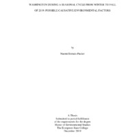
Regular phytoplankton monitoring was conducted at two stations within Budd
Inlet (47.0966° N, 122.9094° W; Fig. 3) located inland, at the southernmost end of the
Puget Sound in Washington state. Station 1 was located at north end (North Point
Landing, 47.0585 W, -122.905119 N) at the estuary head closest to the Deschutes River
and station 2 was at the southern end at mouth of the estuary closest to the south basin of
Puget Sound (Boston Harbor Marina, 47.1400 N, -122.9053 W). These stations were
selected because they represent different environmental conditions for phytoplankton
species diversity and growth. Budd Inlet has been reported to have more dynamic
34
�circulation relative to other bodies of water in Puget Sound (LOTT Waste Management
Partnership, 1998). This increase in mixing is caused by the flow of the Deschutes River,
the second largest river in the Puget Sound and large tidal amplitudes. Station 1 at the
head of the estuary is closest to the river input which, in theory, provides more nutrients
from the river drainage and density stratification due to high fluctuations in salinity.
Station 2 at the mouth is more representative of marine conditions where the salinity is
relatively uniform with depth representing low density stratification.
Figure 3: Two monitoring stations within Budd Inlet, South Puget Sound, WA.
Although the placement of the Deschutes River dam has restricted the flow and
movement of water entering Budd Inlet, this human-induced restriction along with other
anthropogenic activities of dredging and nutrient-loading from local wastewater
35
�treatment plants and runoff into the river has the potential to provoke environmental
consequences to the biota within the local estuarine ecosystem (Ahmed et al., 2019).
The stations were located at the same area of placement as sentinel mussels for
DSP sampling by WDOH. In addition, there is a history of phytoplankton sampling
within Budd Inlet by The Evergreen State College collaborating with SoundToxins in
previous years providing evidence of overall dinoflagellate dominant community at the
estuary head while the mouth was primary a diatom dominant community (G. Chin-Leo,
personal communications, June 15, 2018).
3.2: Research Design: Field Sample Collection and Lab Processing
The study period was from January through October of 2019, which encompassed
the seasonal cycle from winter to fall. At both stations, the frequency of phytoplankton
and water sampling was monthly during winter and fall seasons and weekly during the
spring and summer seasons. Samples were collected to determine cell abundance and
species composition using two different methods.
To determine abundance, the method included quantitatively concentrating
surface waters. Dinophysis, the target species and sometimes dominant species were
counted. Due to the low abundance of Dinophysis spp., in winter, a large amount of
water was concentrated (~15-120 L) using a 20 m mesh phytoplankton net used as a
sieve. The concentrated phytoplankton were condensed further by using a 20 m mesh
sieve with the final concentration ~200-400 mL. Thus, the concentration factor could be
as high as 600 times the normal cell density. The water volume collected for
concentration was adjusted depending on the concentration of cells in natural waters.
During blooms, for example, 15 L were sufficient to produce a dense sample for counts.
36
�The sample for species composition was completed via a vertical tow near or during high
tide; three tows were completed each time to collect enough water for concentration. The
vertical tow allowed for collection of plankton throughout the water column. This was
important because some species migrate vertically or accumulate and density interfaces.
The concentrated phytoplankton was preserved with 2.5% Glutaraldehyde for storage and
possible subsequent Scanning Electron Microscope analysis.
Biological, physicochemical, and water quality parameters were also measured.
Surface seawater samples were collected for phytoplankton biomass (chlorophyll-a) and
nutrient (ammonium, nitrate, silicate, and phosphate) analysis. Measurements of
temperature, salinity, and dissolved oxygen where obtained in situ with a multi-parameter
sensor YSI-2030. Light transparency was measured with the Secchi disk. Coastal Salinity
Index (CSI) was also computed by subtracting the bottom salinity by the surface salinity.
This was used to estimate changes in density stratification.
3.3: Dinophysis Abundance, DSTs, and Environmental Analyses
3.3.1: Dinophysis Abundance and Species Composition
Concentrated phytoplankton samples (~200 mL) were examined with a gridded
Sedgewick Rafter counting chamber and observed on an Olympus BX63 microscope.
Three rows, at a minimum, were chosen randomly and enumerated for the majority of the
concentrated samples so there would be at least ~10 cells per row. The mean counts per
mL were then multiplied by the number of rows on the slide. Dinophysis cells was also
identified to the species level.
For phytoplankton species composition, relative abundance observations were
determined for each genus present. One drop of the species composition sample was
37
�placed on the microscope slide, and the relative abundance was calculated by determining
the percent of species of one genus relative to the total population. The classifications are
as follow: absent (no cells were found), rare (1 cell was found), common (2 cells were
found), and abundant (3 or more cells were found). Dinophysis species and most of the
common phytoplankton were confirmed via light microscopy and scanning electron
methods.
Diarrhetic Shellfish Poisoning (DSP) data was obtained from the WDOH Marine
Biotoxin Monitoring Program. Their sampling procedure is as follows: blue mussels
(Mytilus edulis) were collected bi-weekly on an annual basis at the estuary head and in
summer (May-Sept) at the estuary mouth. Sentinel mussels at these sites were initiated in
2015 and since then have been monitored continuously. WDOH monitors and analyses
the mussel tissue for DSP toxin profile of Okadaic acid, DTX-1, and DTX-2 using the
method of liquid chromatography-mass spectrometer (LC-MS).
3.3.2: Measurements of Environmental Parameters
Seawater samples were collected, frozen, and processed at the laboratory for
quantification of chlorophyll-a and inorganic nutrient concentrations. Triplicate
chlorophyll-a samples were filtered onto a glass fiber filter (Whatman GF/F) and stored
frozen below 0 C. For processing, filters were extracted for 24 hours in 90% high grade
acetone, and filtrate from the chlorophyll-a samples were used for nutrient analysis and
stored in -10 F freezer. The chlorophyll-a was measured with an10-AU Fluorometer
(Parsons et al., 1984).
Nutrient filtrates were analyzed for nitrogen, silicate, phosphate, and ammonium
using the standard methods. Nitrogen (nitrate and nitrite), phosphate, and silicate were
38
�quantified using standard microplate reader colorimetric methods, and the samples were
read by the Molecular Devices VersaMax (Ringuet et al., 2011). Ammonium samples
were analyzed with the orthophthaldialdehyde (OPA) method and read on Turner designs
10-AU (Trilogy) fluorometer (Holmes et al. 1999).
Other physical and meteorological data were obtained. Wind speed/direction, air
temperature, and average precipitation were results reported in Budd Inlet, Olympia by
the NOAA National Weather Service (archived). Deschutes River flow discharge was
also obtained from the U.S. Geological Survey. Solar radiation data was obtained from
the Scientific Computing Weather Station of The Evergreen State College. DSP
concentrations at both of the sample locations were provided by the Washington
Department of Health to determine if toxicity was related to abundance.
3.4: Statistical Analyses
To understand if the environmental parameters measured are related to
Dinophysis abundance, statistical analyses were performed via a simple linear regression,
where the abundance is the response variable while the environmental parameter is the
independent variable. Log transformations to the Dinophysis abundance data were
executed to meet the assumptions of normality to run the test. The best way to deal with
heteroscedastic and skewed results is by using a log transformation of the data
(Hattenrath-Lehmann et al., 2013).
In order to run regression, the data has to meet the assumption of linearity. To
meet this assumption, I performed sensitivity testing of the data at both the head and
mouth. The log transformation was used to reduce the skew of dependent and
independent variables because they are not necessarily linear in nature. I also ran the tests
39
�without the transformation and compared the results and found that the regression
analysis showed different significant outcomes related to abundance at the head of the
estuary, but not at the mouth. This may mean that the non-transformed data from the
estuary head was more skewed than the data obtained from the estuary mouth since the
larger density blooms occurred. Independent t-tests were run to determine if the
differences in biological, meteorological, and water quality parameters between the
estuary head and mouth.
In addition to the statistical analysis, qualitative analyses of Dinophysis densities
and environmental parameters were also performed. Time series graphs were analyzed to
assist in the evaluation of possible delays in environmental conditions, especially since
the statistical relationships potentially do not fully represent the lag time between the
response of Dinophysis to the environmental factors.
40
�CHAPTER 4: RESULTS
4.1: Phytoplankton Species Composition
Phytoplankton species composition varied over the study period. For simplicity, I
will refer to the mouth of the estuary as BHM (Station 1) and NPL (Station 2) as the
head. NPL exhibited high species richness of species, and a total of 75 species were
observed with diatoms dominating throughout the majority of the year, with the
exception of summer months when dinoflagellates dominated. NPL had lower species
richness with a total of 63 species. Both stations had a total 23 species of dinoflagellates,
and the remaining were diatom species. About 34.8% of the species observed were
dinoflagellates and 65.2% were diatoms. The estuary head also exhibited a similar
pattern: 32.9% of the species were dinoflagellates and 67.1% were diatoms. Although
species richness was similar at both stations, overall there was a greater relative
abundance of diatoms at BHM while more dinoflagellates were present at NPL. About
4% of the species were commonly found throughout the study, being detected greater
than 20 times at the estuary head, and 3% of common species were found at the estuary
mouth.
Diatoms dominated winter to late spring (January to early June) and
dinoflagellates dominated summer to fall (early June to October). There was a difference
in species composition between sites. NPL’s most abundant species was Ceratium fusus
and most common was Chaetoceros debilis. The most abundant species was C. debilis
and most common species was Skeletonema costatum at BHM. Several diatoms and
dinoflagellates were present but were considered rare because they were observed
infrequently at very low concentrations. Also, there were several HAB species found
41
�throughout the study including: Pseudo-nitzschia spp., Alexandrium spp., Dinophysis
spp., Heterocapsa triquetra, and Protoceratrium reticulatum. Dinophysis spp. and
Pseudo-nitzschia spp. were the two dominant HAB species, often co-occuring throughout
the seasonal cycle at both stations. Other harmful but non-toxic algae, Ceratium fusus and
Akashiwo sanguinea, were found to co-occur with Alexandrium spp. (see Appendix A).
4.2: Spatiotemporal Differences
There were significant differences (p < 0.05, n = 55) between both stations in the
following parameters averaged over the study period, including: dissolved oxygen,
ammonium concentrations, silicate concentrations, transparency (Secchi depth), surface
water temperature at 1m depth, and coastal salinity index (Table 1). Nutrient ratios,
nitrate concentrations, phosphate concentrations, and salinity at 1m depth were not found
to be statistically significant.
Biomass levels were not significantly different between both sites (Table 1).
Biomass of phytoplankton as estimated from chlorophyll-a varied from 0.78 mg of
seawater/L seawater to 58.2 mg of seawater/L with maximal values on 9/7/19 at NPL
(Fig. 4). Chlorophyll-a ranged from 1.55 to 14.78 mg of seawater/L with highest
concentrations occurring on 7/2/19 at BHM (Fig. 5).
42
�Table 1: Differences in environmental parameters between the estuary head and estuary
mouth (significant p-values are boldfaced).
Figure 4: Time series of biomass (chlorophyll-a) levels throughout the annual seasonal
cycle at the estuary head (NPL) in Budd Inlet.
43
�Figure 5: Time series of biomass (chlorophyll-a) levels throughout the annual seasonal
cycle at the mouth of the estuary (BHM) in Budd Inlet.
Biomass was significantly related to nitrate (NO3-) at both stations
(estuary head: p = 0.0004, r 2 = 0.36; estuary mouth: p = 0.002, r 2 = 0.37) and
phosphate (PO4-) (p = 0.002, r 2 = 0.30) at the estuary head. To determine how changes
in nutrient composition might affect species composition, I computed the ratios of total
nitrogen to phosphorous and silica to nitrogen and determined if changes in these ratios
were related to biomass. Using simple linear regression, two nutrient ratios were
correlated to chlorophyll-a concentrations. Nutrient ratios of DIN:DIP are a significant
factor at both stations (NPL: p = 4.15x10⁻⁵; r 2 = 0.46; BHM: p = 0.002, r 2 =
0.37) (Table 2). In addition, the ratios of DSI:DIN were found to be significant at both
stations (NPL: p = 6.1x10⁻⁵ , r 2 = 0.44; BHM: p = 8x10⁻³ , r 2 = 0.29) (Table 2).
44
�Table 2: Regression analysis between biomass and environmental parameters at the
estuary head (NPL) and mouth (BHM) in Budd Inlet (significant p-values are boldfaced).
4.3: Dinophysis Species Diversity and Abundance
Dinophysis species were present throughout the study at both stations.
Dinophysis was not detected once in 34 weeks of sampling at the head of the estuary
station. At the estuary mouth, Dinophysis was observed in all the 31 weeks monitored.
Dinophysis was found to be both abundant and dominant during the peak densities in
summer months at both sites. During the blooms, Dinophysis was co-occurring with other
diatoms, primarily Thalassiosira spp. The relative abundance of Dinophysis was largely
considered rare and occasionally common during all other months during the spring,
45
�summer, and fall. Dinophysis typically co-occurred with another HAB diatom genus,
Pseudo-nitzschia.
D. norvegica was the most abundant Dinophysis species at both sites, reaching
densities of 23,857 cells/L at the estuary head and 3,590 cells/L at the estuary mouth on
6/6/19. Other species observed during the study included: D. acuminata, D. fortii, D.
rotundata, D. odiosa, and D. parva. Their abundances were much lower with the largest
densities of 1,933 cells/L of D. fortii (9/13/19), 542 cells/L of D. acuminata (10/2/19), 71
cells/L of D. odiosa (8/7/19), 30 cells/L of D. rotundata (8/31/19), and 50 cells of D.
parva (8/13/19) at the station near the head of the estuary. At the estuary mouth,
abundances of Dinophysis were considerably lower reaching densities of 115 cells/L for
D. acuminata (6/6/19), 67 cells/L of D. fortii (6/6/19), 84 cells/L of D. rotundata
(7/2/19), 318 cells/L of D. odiosa (7/18/19), and 1 cell/L of D. parva (9/7/19). For most
of the year, D. norvegica, D. acuminata, and D. fortii co-occurred at both sites.
4.4: Spatiotemporal Distribution of Dinophysis Species
Maximal densities of Dinophysis illustrated a similar correspondence at both of
the sites during the summer months (Fig. 6). Variations of abundance were considerably
noticeable at both sites from June to August. The major difference is that the
concentrations vary more widely at the head of the estuary showing the highest values of
Dinophysis abundance. Generally speaking, Dinophysis densities greater than 1,000
cells/L are considered blooms (Macknenzie, 2019). The majority of the Dinophysis
blooms occurred during the summer months at both sites but were also seen during the
fall months at the estuary head.
46
�There were at total of 13 bloom events at NPL and 6 events at estuary head
(BHM) (Fig. 6). There were distinct peaks in Dinophysis abundance in the summer
months from early June to late July at both stations. A total of four dense blooms
occurred at the estuary head on 6/6/19, 6/23/19, 7/11/19, and 7/24/19 (Fig. 3). At the
estuary mouth there were three peaks occurring on 6/6/19, 6/23/19, and 7/18/19. Maximal
values occurred at both locations on two occasions during the early summer (6/6/19 and
6/23/19). Dinophysis abundance ranged from 1 cell/L to 33,600 cells/L with highest
abundance on 6/27/19 at the head of the estuary. Also at the NPL station near the estuary
mouth, Dinophysis densities ranged from 1 cell/L to 3,705 cells/L with the highest
density occurring on 6/6/19. Dinophysis was the dominant species during the peak
blooms. The relative total of the entire Dinophysis species was considered abundant
during these summer months starting in June to August at both sites, although other
diatoms co-occurred but were relatively rare in abundance.
47
�Figure 6: Dinophysis abundance over the seasonal cycle from winter to fall of 2019 at the
estuary head (NPL) and mouth (BHM) in Budd Inlet, WA.
4.5: Influence of Environmental Conditions on the Distribution of Dinophysis
Regression and qualitative analyses were evaluated to determine whether there is
a relationship between biomass and Dinophysis densities. At the estuary head, Dinophysis
abundance was significantly related to biomass, but not at the mouth (p = 0.02, r 2 =
0.17) (Table 3). The biomass (chlorophyll-a concentrations) demonstrated two different
patterns in relation to the Dinophysis blooms. NPL biomass levels ranged from 2.6 to
11.3 mg/L of seawater during the summer bloom period (May to July). As the densities
of the blooms decreased, the chlorophyll-a concentrations increased, showing a positive
48
�relationship. BHM had a variable biomass from 3.9 to 13.9 mg/L of seawater during the
same duration, not demonstrating any particular pattern related to abundance.
The estuary head biomass was relatively low in the winter and spring. During the
summer, biomass increased as the Dinophysis bloom abundances decreased. There was a
considerable increase in chlorophyll-a concentrations during the late summer and early
fall. On the other hand, the estuary mouth presented an overall increase in biomass
throughout the four seasons. At NPL, the biomass decreased to 1.7 mg/L of seawater
during the biggest Dinophysis bloom on 6/6/19.
Table 3: Independent means t-test statistical analysis of Dinophysis abundance related to
biomass (chlorophyll-a) (significant p-values are boldfaced).
Linear regression was used to test if nutrients explained the timing and magnitude
of blooms. In addition to the importance of elemental composition for the stimulation of
Dinophysis blooms, it is also important to understand the composition of nutrient ratios.
Nutrient composition not just magnitude can affect phytoplankton growth. Investigating
these nutrient ratios characterizes their role in shaping phytoplankton assemblages,
specifically focusing on the dinoflagellate community with a dominance of HAB species
(i.e. Dinophysis spp.).
The Redfield-Belinksi ratio of 106:15:16:1 represents the total dissolved
inorganic nutrient composition of carbon to nitrogen to silica to phosphate
(DIC:DSI:DIN:DIP) available for phytoplankton utilization via the biogeochemical
cycling of nutrients (Choudhury & Bhadbury, 2015). I wanted to analyze the relationship
49
�between abundance and nutrient composition, therefore, I choose to analyze the
composition by evaluating the ratios. I computed the following nutrient ratios of
DIN:DIP, DSI:DIN, and DSI:DIP to examine if there are deviations from the standard
nutrient ratios to influence dinoflagellate assemblages, specifically focusing on
Dinophysis abundances.
For the total dissolved inorganic nitrogen, I included both ammonium and nitrate
concentrations but have omitted the analysis of nitrite because of the lack of equipment to
quantify the concentrations, which is usually a very small fraction of the total inorganic
in nature. Specifically, we are looking at deviation from nutrient ratios which is looking
at ratios at which cells are made.
I tested the relationship of abundance with nutrients, but the regressions don’t
capture that possible delay between nutrient changes to which the phytoplankton respond.
To examine the possible connection between the changes in one or the other that, I
analyzed how the nutrients varied around the time of the blooms via time series data to
see the correspondence of changes in the various parameters.
Dinophysis abundance at the head of the estuary was negatively related to
nitrate (p = 0.01, r 2 = 0.19) and positively related to phosphate (p = 0.0006, r 2 =
0.33) concentrations. Dinophysis abundance was not significantly related to ammonium
and silicate. At the mouth of the estuary, all four nutrients measured were not
significantly related to Dinophysis abundance (Table 4).
50
�Table 4: Simple linear regression analysis of Dinophysis abundance related to nutrients
(nitrate, ammonium, silicate, and phosphorous) at the estuary mouth (NPL) and head
(BHM) in Budd Inlet (significant p-values are boldfaced).
The phosphate concentrations at the estuary head ranged from 0.8 to 4.6 M and
1.1 to 5.7 M at the estuary mouth (Fig. 7; Fig. 8) and levels were low throughout the
winter and considerably higher throughout the summer and fall. The time series shows
that the peak concentrations of phosphate overlap with the Dinophysis blooms in the
summer from June to the end of August (Fig. 9). The time series graphs for the estuary
head shows that during the peak blooms from June to September, the phosphate
concentrations were greater than in winter. Also, the estuary mouth shows phosphate
concentrations were low in the first half of the spring season, while the second half shows
a pulse of phosphate reaching maximal value of 5.7 M on 5/15/19 (Fig. 10). Shortly
after the surge, there was a sharp decline of phosphate to 1.1 M. A bloom of Dinophysis
followed two weeks after the steep decline in phosphate. During the peak blooms,
phosphate concentrations remained low until the blooms declined. After the blooms
ceased, the phosphate levels increased.
51
�Figure 7: Time series of phosphate levels over the seasonal cycle of winter to fall of 2019
at the estuary head (BHM) in Budd Inlet.
Figure 8: Time series of phosphate levels over the seasonal cycle of spring to fall of 2019
at the estuary mouth (NPL) in Budd Inlet.
52
�Figure 9: Time series of Dinophysis abundance versus phosphate levels at the estuary
head (NPL) in Budd Inlet.
Figure 10: Time series of Dinophysis abundance versus phosphate levels at the estuary
mouth (BHM) in Budd Inlet.
53
�At the estuary head, nitrate concentrations were noticeably higher in the winter
and spring (Fig. 11). In summer, nitrate levels were low and increased in the fall. Before
the blooms occurred, nitrate levels were very high. During the bloom, the nitrate
concentrations decreased while Dinophysis abundances increased (Fig. 12). Also, the
mouth of the estuary shows a similar trend during the spring, summer bloom season, and
fall (Fig. 13). The peak of Dinophysis abundances occurred a few weeks after the
elevated levels of nitrate were present (Fig 14).
Figure 11: Time series of phosphate levels over the seasonal cycle of spring to fall of
2019 at the estuary head (NPL) in Budd Inlet.
54
�Figure 12: Time series of Dinophysis abundance versus nitrate levels at the estuary head
(NPL) in Budd Inlet.
Figure 13: Time series of phosphate levels over the seasonal cycle of spring to fall of
2019 at the estuary head (NPL) in Budd Inlet.
55
�Figure 14: Time series of Dinophysis abundance versus nitrate levels at the estuary mouth
(BHM) in Budd Inlet.
In addition, Dinophysis abundance at NPL was significantly related to nutrient
ratios of dissolved inorganic nitrogen to dissolved inorganic phosphate (DIN:DIP)
(p = 0.014, r 2 = 0.19)and dissolved silica to dissolved inorganic phosphate (DSI:DIP)
(p = 0.01, r 2 = 0.19) (Table 5). On the other hand, the estuary mouth was not
significantly related to any of the nutrient ratios. The DIN ratios only consist of
ammonium and nitrate concentrations due to lack of equipment at this time to determine
nitrite levels. However, it is known that nitrite is a small fraction of the total
concentrations thus should have minor influence in the ratio.
56
�Table 5: Simple linear regression analysis of Dinophysis abundance related to nutrients
ratios at the estuary mouth (NPL) and head (BHM) in Budd Inlet.
The nutrient ratio of DSI:DIP ranged from 0.4 to 21.4 with maximal values
occurring during the winter to spring at the estuary head (Fig. 15; Fig 16). The ratios
decreased in early June to August, the same periods when the peak blooms occurred (Fig.
17). Similar occurrences appeared at the mouth of the estuary: when Dinophysis densities
were low, DSI:DIP ratios were high (Fig. 18). However, when cell densities were high,
the ratios decreased. A large inversion peak occurred at the same time the largest bloom
occurred on 6/6/19. Overall, the nutrients ratios were higher and more variable at the
head of the estuary compared to the mouth.
57
�Figure 15: Time series of nutrient ratios of dissolved silica to dissolved inorganic
phosphate (DSI:DIP) over the seasonal cycle of spring to fall of 2019 at the estuary head
(NPL) in Budd Inlet.
Figure 16: Time series of nutrient ratios of dissolved silica to dissolved inorganic
phosphate (DSI:DIP) over the seasonal cycle of spring to fall of 2019 at the estuary
mouth (BHM) in Budd Inlet.
58
�Figure 17: Time series of Dinophysis abundance versus nutrient ratios of dissolved silica
to dissolved inorganic phosphate (DSI:DIP) at the estuary head (NPL) in Budd Inlet.
Figure 18: Time series of Dinophysis abundance versus nutrient ratios of dissolved silica
to dissolved inorganic phosphate (DSI:DIP) at the estuary mouth (BHM) in Budd Inlet.
59
�Nutrient ratios of DIN:DIP ranged from 0.4 to 21.6 at the estuary head (Fig. 19).
Ratios were elevated during the winter to the end of spring. When the summer season
ensued, a sharp decline in DIN:DIP occurred on 6/1/19 and very low ratios of DIN:DIP
remained low thru the fall. Shortly after this decline of phosphate levels, the first bloom
followed on 6/6/19 (Fig. 20). In contrast, the mouth of the estuary showed a gradual
decline in the DIN:DIP ratios over spring to end of the summer (Fig. 21). Ratios
decreased when the blooms were present.
Figure 19: Time series of nutrient ratios of dissolved inorganic nitrogen to dissolved
inorganic phosphate (DIN:DIP) over the seasonal cycle of spring to fall of 2019 at the
estuary head (NPL) in Budd Inlet.
60
�Figure 20: Time series of Dinophysis abundance versus nutrient ratios of dissolved
inorganic nitrogen to dissolved inorganic phosphate (DIN:DIP) at the estuary head (NPL)
in Budd Inlet.
Figure 21: Time series of nutrient ratios of dissolved inorganic nitrogen to dissolved
inorganic phosphate (DIN:DIP) over the seasonal cycle of spring to fall of 2019 at the
estuary mouth (BHM) in Budd Inlet.
61
�Figure 22: Time series of Dinophysis abundance versus nutrient ratios of dissolved
inorganic nitrogen to dissolved inorganic phosphate (DIN:DIP) at the estuary mouth
(BHM) in Budd Inlet.
Although the relationship between ammonium and Dinophysis abundance was not
statistically significant, both stations exhibited elevated levels of ammonium during the
spring before the Dinophysis blooms. Ammonium levels were substantially greater at the
head of the estuary relative to the mouth, reaching maximal levels of 12.0 M (Fig. 23).
The estuary head time series showed moderate levels of ammonium in winter, then
increased throughout spring until beginning of summer (6/6/19). As summer progressed,
ammonium concentrations declined from 11.0 M to 0.3 M from 6/6/19 to 8/1/19. This
decline in ammonium concentrations during the summer months corresponded with the
high-density blooms of Dinophysis at both stations between 6/6/19 to 7/24/19 (Fig. 24).
The levels decrease in accordance with decreasing bloom activity until 8/1/19. In
comparison, ammonium concentrations were significantly lower at the estuary mouth
(Fig. 25). Spring showed a similar trend with highest levels of ammonium concentrations
62
�ranging from 1.1 M to 4.4 M during 3/17/19 to 5/23/19. Levels of ammonium
decreased after the first bloom on 6/1/19. The lowest ammonium concentrations occurred
on 8/1/19 directly after the last bloom of the summer season (Fig. 26).
Figure 23: Time series of ammonium levels over the seasonal cycle of spring to fall of
2019 at the estuary head (BNPL) in Budd Inlet.
63
�Figure 24: Time series of Dinophysis abundance versus ammonium levels at the estuary
head (NPL) in Budd Inlet.
Figure 25: Time series of ammonium levels over the seasonal cycle of spring to fall of
2019 at the estuary mouth (BHM) in Budd Inlet.
64
�Figure 26: Time series of Dinophysis abundance versus ammonium levels at the estuary
mouth (BHM) in Budd Inlet.
Each of the water quality and meteorological factors were measured and analyzed
in order to examine the how environmental conditions might influence Dinophysis
densities. Analyses of simple linear regressions and time series were performed. There
were statistically significant correlations (p < 0.05) between Dinophysis abundance and
changes in environmental conditions. At the head of the estuary, Dinophysis abundance
was significantly related to dissolved oxygen (r 2 = 0.19), surface water temperature at
1m depth (r 2 = 0.44), air temperature (r 2 = 0.32), river discharge (r 2 = 0.51), and
solar radiance (r 2 = 0.17) (Table 6; Table 7). River discharge and surface water
temperature were the largest contributors to Dinophysis abundance at NPL. In
comparison, the station at the estuary mouth was significantly (p < 0.05) related to
salinity (r 2 = 0.28), surface water temperature (1m depth) (r 2 = 0.18), air
65
�temperature (r 2 = 0.27), river discharge (r 2 = 0.31), wind speed (r 2 = 0.15), and solar
radiance r 2 = 0.19) (Table 6; Table 7). River discharge and salinity were the most
significant factors at BHM.
Table 6: Simple linear regression analysis of Dinophysis abundance related to
meteorological conditions at the estuary mouth (NPL) and head (BHM) in Budd Inlet.
Table 7: Simple linear regression analysis of Dinophysis abundance related to water
quality parameters at the estuary mouth (NPL) and head (BHM) in Budd Inlet (significant
p-values boldfaced).
66
�Dissolved oxygen was qualitatively analyzed via time series plots to understand if
the levels decreased during the Dinophysis blooms periods. Levels of dissolved oxygen
were highly variable throughout the seasonal cycle at the estuary head ranging from 3.60
to 10.2 mg/L (Fig. 27). High levels occurred during the winter, spring, and fall. In the
summer, when Dinophysis reached peak densities, dissolved oxygen levels greatly
decreased (Fig. 28). The second peak bloom shows dissolved oxygen made very sharp
declines, reaching low of 3.60 mg/L on 7/2/19. Dissolved oxygen levels at the estuary
mouth were relatively stable in contrast to the head, staying within the range of 6.25 to
9.99 mg/L (Fig. 29). The dissolved oxygen levels did show slight decline from 9.99 to
7.33 in when high Dinophysis abundances were present (Fig. 30).
Figure 27: Time series of dissolved oxygen levels over the seasonal cycle of spring to fall
of 2019 at the estuary mouth (BHM) in Budd Inlet.
67
�Figure 28: Time series of Dinophysis abundance versus dissolved oxygen levels at the
estuary head (NPL) in Budd Inlet.
Figure 29: Time series of dissolved oxygen levels over the seasonal cycle of spring to fall
of 2019 at the estuary mouth (BHM) in Budd Inlet.
68
�Figure 30: Time series of Dinophysis abundance versus dissolved oxygen levels at the
estuary mouth (BHM) in Budd Inlet.
Surface water and air temperatures were evaluated to determine whether warm
waters prevent mixing, allowing algae to growth densely. With lack of mixing, cells can
become concentrated locally in the waters. Air and surface water temperatures (1m
depth) followed the same trend of gradually increasing in temperature from the period of
winter to summer then a decline in fall at the head of the estuary (Fig. 31). The mouth of
the estuary showed similar appearances in temperatures from winter to spring, however
the surface water temperatures remained fairly stable in the fall (Fig. 32). Dinophysis
abundances coincide with the rising surface water temperatures at both stations (Fig. 33).
During the winter to spring, surface water temperature increased from 7.7C to 13.6C
between 3/7/19 and 6/1/19. The first two blooms occurred during surface water
temperatures of 13.3C to 13.6C. Second set of blooms happened when temperatures
increased ranging from 14.7C to 15C. On the other hand, a similar pattern was
69
�displayed at the mouth of the estuary. In a similar trend, the first peak bloom at the
estuary mouth coincided after the primary increase in surface water temperatures from
winter (2/20/19) to early June (6/1/19) ranging from 8C to 14.2C (Fig. 34). The other
two peak blooms corresponded with higher temperatures: second peak bloom at 13.6C
and third peak blooms at 14.9C.
Figure 31: Time series of air and surface water temperatures over the seasonal cycle of
spring to fall of 2019 at the estuary head (NPL) in Budd Inlet.
70
�Figure 32: Time series of air and surface water temperatures (1m depth) over the seasonal
cycle of spring to fall of 2019 at the estuary mouth (BHM) in Budd Inlet.
Figure 33: Time series of Dinophysis abundance versus surface water temperatures (1m
depth) at the estuary head (NPL) in Budd Inlet.
71
�Figure 34: Time series of Dinophysis abundance versus surface water temperatures (1m
depth) at the estuary mouth (BHM) in Budd Inlet.
River discharge plays a major role in the biogeochemical cycling of estuaries
which are critical in the circulation of the waters and provide nutrient loading of
inorganic compounds that are essential for instating blooms and shaping phytoplankton
community structure. In addition to the statistical analysis, time series represented the
form and magnitude of the Deschutes River discharge relative to Dinophysis abundance.
The placement of the river adjacent to NPL relative to BHM might be a major factor
explaining the larger density blooms at NPL.
River discharge presented high levels in the winter to mid-spring (1/13/19 to
4/18/19) ranging from 273 ft 3 / sec to 662.7 ft 3 /sec (Fig. 31). After 4/18/19, there was a
major decline in river outputs during the summer and fall (Fig. 35). Dinophysis
abundances at both stations coincide with low levels of river discharge from June to end
of August (Fig. 36; Fig 37).
72
�Figure 35: Time series of the Deschutes River discharge into Budd Inlet during the
seasonal cycle of winter to fall of 2019.
Figure 36: Time series of Dinophysis abundance versus river discharge at the estuary
head (NPL) in Budd Inlet.
73
�Figure 37: Time series of Dinophysis abundance versus river discharge at the estuary
mouth (BHM) in Budd Inlet.
Wind can influence the phytoplankton activity by concentrating or diluting the
dispersal of phytoplankton; therefore, time series of wind speed with direction were
evaluated to determine if there is a relationship to Dinophysis abundance. Wind speed
and direction in Budd Inlet varied considerably throughout the study period (Fig. 38).
Shifts in wind direction from north to south, along with increases in wind speed overlap
with two major peaks densities of Dinophysis at both stations (Fig. 39; Fig 40).
74
�Figure 38: Time series of the wind speed and direction in Budd Inlet during the seasonal
cycle of winter to fall of 2019.
Figure 39: Time series of Dinophysis abundance versus wind speed at the estuary head
(NPL) in Budd Inlet.
75
�Figure 40: Time series of Dinophysis abundance versus wind speed at the estuary mouth
(BHM) in Budd Inlet.
Solar radiation is one of the main factors for phytoplankton growth.
Phytoplankton are able to absorb light, in turn promoting warmer conditions in the
surface water as well as prompt algal blooms. Solar radiation was variable but gradually
increased during the winter to spring. Highest levels of solar radiation appeared during
5/23/19 to 6/23/19 ranging from 257.6 to 289.0 W/m2 and between 7/18/19 to 8/13/19
ranging from 208.3 W/m2 to 290.4 W/m2 (Fig. 41). At the estuary head, the peak of
solar radiation corresponded during the two primary Dinophysis blooms events during
May to June corresponds; however, the other bloom events show correspondence with
the second phase in elevated total radiation emittance from July to August (Fig. 42).
Similarly, at the estuary mouth the two main peaks of Dinophysis blooms correlate with
increased levels of solar radiation in the first half of the summer along with the third peak
bloom in the second half (Fig. 43).
76
�Figure 41: Time series of solar radiation in Budd Inlet during the seasonal cycle of winter
to fall of 2019.
Figure 42: Time series of Dinophysis abundance versus solar radiation at the estuary head
(NPL) in Budd Inlet.
77
�Figure 43: Time series of Dinophysis abundance versus solar radiation at the estuary
mouth (BHM) in Budd Inlet.
Water transparency was measured via Secchi depth to understand the depth to
which the light penetrates the water. Light penetration is an important component to
phytoplankton growth because it is necessary for activities of photosynthesis. Water
transparency (Secchi depth at 1m) ranged from 1.8 m to 5.8 m at the estuary mouth.
While the head of the estuary ranged from 2.9 m to 5.6 m, water transparency was not
qualitatively nor statistically related to Dinophysis abundance.
Time series between Dinophysis abundance and rainfall were analyzed with
respect to the possible lag time between the input of the rain and the response time from
Dinophysis. Rainfall events are potential important contributors to inputs of dissolved
inorganic nutrients in the estuaries that can support phytoplankton growth and activity.
Rainfall showed maximal values in the winter (0.04 m) and fall (0.02 m) (Fig. 44). While
the early spring season exhibited moderate levels of rainfall reaching up to 0.42 in, lowest
levels of rainfall occurred during late spring into the end of the summer season. High
78
�levels of rainfall coincided with low densities of Dinophysis at both stations (Fig. 45). At
both the estuary head and mouth, blooms developed in the summer months after a period
of low precipitation. There was a peak of 0.13 inches of rainfall on 7/2/19 between the
two initial Dinophysis blooms and the remaining blooms at both stations. In addition,
rainfall also displayed potential influences on ammonium concentrations throughout the
seasonal cycle. At the estuary head, concentrations of ammonium remained at low levels
during the winter and considerably increased during the summer (Fig. 46). The estuary
mouth showed increasing levels of ammonium during the summer (Fig. 47). The
concentrations were considerably lower than the estuary head after the rainfall periods
occurred.
Figure 44: Time series of solar radiation in Budd Inlet during the seasonal cycle of winter
to fall in 2019.
79
�Figure 45: Time series of Dinophysis abundance versus average rainfall at the estuary
head (NPL) in Budd Inlet.
Figure 46: Time series of Dinophysis abundance versus average rainfall at the estuary
mouth (BHM) in Budd Inlet.
80
�Figure 47: Time series of average rainfall and ammonium levels at the estuary head
(NPL) during the seasonal cycle of winter to fall in 2019.
Figure 48: Time series of average rainfall and ammonium levels at the estuary mouth
(BHM) during the seasonal cycle of winter to fall in 2019.
81
�4.6 Shellfish Toxicity
A way to monitor for biotoxins is to measure diarrhetic shellfish poisoning
(DSP) toxins in mussel tissues. Mussels filter a tremendous amount of water, thus
concentrating the algal toxins. WDOH routinely collects mussels (sentinel mussels) and
analyzes their tissues for algal toxins. WDOH collected, processed, and analyzed blue
mussel tissue samples for okadaic acid, dinophysistoxin-1 (DTX-1), and dinophysistoxin2 (DTX-2) at both stations. Dinophysis enumeration was completed within ±48 hours
(majority of samples) of the time the DSP toxin sampling was completed. This generates
data that allows the WDOH to manage the closures of shellfish beds for harvesting when
toxin levels pass given minimum concentrations. Total diarrhetic shellfish toxins were
statistically and quantitively analyzed.
While DSP toxins are generated by Dinophysis, its abundance and DSP in toxins
may not coincide in time. This is because the concentration of toxin by mussels occurs
over an unknown period of time. The same toxin level, for example, could be achieved by
filtering small concentrations of cells over a long period of time, or by consuming a large
concentration of cells over a short period of time. Furthermore, mussels can get rid of the
toxin following continued filtration (depuration) of non-toxic cells. If a Dinophysis
bloom occurs following depuration, there will not be a relationship between abundance
and toxins in mussels (Svensson, 2003). In the context of this study and an additional
complication is that the WDOH data was collected at much longer time intervals than the
abundance data. Given that WDOH provided the DSP data and in spite of these issues
described, I ran linear regression analysis to evaluate if there is a relationship between
Dinophysis abundance and DSP.
82
�There were 20 samples from January to the end of September at NPL with DSP
concentrations ranging from 0.50 to 9 𝜇g/100g (Fig. 49). There were 11 samples
collected at BHM from mid-May to end of September with DSP concentrations ranging
from 0.24 to 1.16 𝜇g/100g (Fig. 50). Three samples were taken around the time of
Dinophysis blooms. The highest DSP levels were located at NPL, occurring on March 20.
These high DSP levels occurred in the mid-spring before the summer bloom period.
During the bloom period, there was also another minor peak in the month of June
reaching a maximal DSP level of 3.52 𝜇g/100g.
Levels of DSP toxins were very low over the seasons at both stations—not
reaching the USDA action level of 16 g/100g. The majority of the DSP toxin present
was DTX-1, and minimal levels of okadaic acid were present throughout the study.
Dinophysis abundance and DSP toxin concentrations from WDOH (Table 8) were not
significantly related.
Figure 49: Time series of Dinophysis abundance versus the total DSP toxin levels at the
estuary head (NPL) during the seasonal cycle of winter to fall in 2019.
83
�Figure 50: Time series of Dinophysis abundance versus the total DSP toxin levels at the
estuary mouth (BHM) during the seasonal cycle of winter to fall in 2019.
Table 8: Regression analysis between Dinophysis abundance versus DSP toxins at the
estuary head and mouth in Budd Inlet (significant p-values are boldfaced).
84
�CHAPTER 5: DISCUSSION
5.1: Overview of Research Questions & Hypotheses
This is this the first study to characterize Dinophysis bloom activity with high
frequency sampling of biological and environmental parameters over a 10-month period
in Budd Inlet, Puget Sound, Washington. The high concentration method was developed
because Dinophysis was reported to be rare in this area particularly in winter. This
method was critical to determining the changes in the abundance and distribution over
space and time of six toxic Dinophysis species. My research questions were: What is the
spatiotemporal distribution of Dinophysis between the estuary head (near Deschutes
River) and the mouth (near south sound basin) over the seasonal cycle from winter to fall
of 2019 in Budd Inlet? What environmental factors control the abundance of Dinophysis
during the study period?
I hypothesize that the station near the head of the estuary would have greater
phytoplankton abundance relative to the mouth. The station adjacent to the Deschutes
river may be more heavily influenced by the river discharge which might support the
notion of elevated nutrient loading and high density stratification that promote an
increase dinoflagellate bloom activity.
The hypothesis also recognizes several meteorological and water quality factors
that were related to Dinophysis abundance and timing of blooms. Availability of nitrogen,
ammonium, and phosphorous were considered to be major factors controlling abundance
of Dinophysis or of its prey (Hattenrath-Lehmann et al., 2015; Gao et al, 2011).
Dinophysis cells are mixotrophic usually predating on Myrionecta rubra but can be
autotrophic when starved. River discharge was hypothesized to be another factor
85
�contributing to Dinophysis blooms because in addition to being a source of nutrients, the
freshwater contributes to creating a stratified water column, which tends to benefit
dinoflagellates (Sellner et al., 2011; Gentien et al., 2015).
Now, I will discuss how my findings provide answers to the research questions. In
this discussion, I will provide an overview of the phytoplankton species composition and
biomass. Then, I will discuss what I found regarding the distribution of Dinophysis both
spatially and temporally and the environmental factors that may explain these trends. In
closing, suggestions for future Dinophysis research are mentioned.
5.2: Phytoplankton Species Composition and Biomass
Diatom species dominated in winter and dinoflagellates species dominated in
spring to summer. This is consistent with the general concept of a shift from diatom to
dinoflagellates when transitioning from cooler to warmer seasons of the year in other
temperate estuaries similar to Budd Inlet. Although the species richness was similar at
both sites, each station species’ evenness varied with higher cell abundance of
dinoflagellates species at the head of the estuary. Dinoflagellate (including Dinophysis
spp.) domination occurs because they benefit from the stratified conditions that are more
common at the head of the estuary due to its proximity to the river (Mackenzie, 2018;
Mena et al., 2019).
Phytoplankton biomass as estimated by chlorophyll-a was only related to
Dinophysis abundance at the head of the estuary. This was most likely due to diatoms
which have more chlorophyll-a content per cell, are generally larger, and more abundant
at the mouth of the estuary.
86
�5.3: Spatiotemporal Distribution of Dinophysis spp.
The results show 4 out of 13 toxic species of Dinophysis are commonly found in
Budd Inlet, Puget Sound. Using a high concentration method, Dinophysis was detected
throughout the four seasons at both stations. In the winter, Dinophysis mainly comprised
D. norvegica, D. acuminata, and D. fortii, while the late spring throughout the summer
was dominated by D. norvegica. D. norvegica was the most common Dinophysis species
found at both locations in all but one week. The density of Dinophysis norvegica blooms
increased during the summer months. This indicates that summer has optimal conditions
for D. norvegica growth, allowing it to outcompete other species. When Dinophysis
bloomed, few other phytoplankton genera were observed. These results are consistent
with D. norvegica blooms on the Pacific Coast of Canada that reached cell densities
exceeding 5x10⁵ cells/L (Hattenrath-Lehmann et al., 2013).
The densities of Dinophysis did not support my hypothesis because the
dominance of D. norvegica was unexpected and D. acuminata has been the most
prevalent species of Dinophysis in Puget Sound and United States, responsible for DSP
outbreaks (Trainer et al., 2013). Dinophysis norvegica has been associated with DSP
outbreaks but these are not as extensive as DSP events associated Dinophysis acuminata
blooms. To date, D. norvegica is not known to be a major contributor to DSP outbreaks
in cold-temperate waters and the DSP events it causes have been mild.
Dense cell abundances of D. norvegica were found at the estuary head relative to
the mouth. At the head, D. norvegica co-occurred more frequently with D. acuminata and
D. fortii. These two species have been known to produce diarrhetic shellfish toxins
87
�(DSTs) that cause extensive DSP outbreaks. Their abundance at the head may result from
hydrographic conditions of strong thermal water-column stratification during late spring
and early summer which seem to favor cell densities of Dinophysis (Delmas et al., 1992;
Reguera et al., 1995; Godhe et al., 2002; Hattenrath-Lehmann et al., 2015).
5.4 Dinophysis Abundances and Environmental Factors
In this study, several environmental factors were examined to understand the
bottom-up control of Dinophysis abundance. These included water quality and
meteorological variables.
The question of whether nutrient loading contributes to Dinophysis blooms has
not been addressed extensively in the literature because Dinophysis is mixotrophic.
Nutrients, however, can be important because they are needed by Dinophysis prey and
also by D. acuminata and D. fortii when starved. I considered the nutrients needed for
phytoplankton growth and computed various nutrient ratios to explore if variations in
nutrient composition are important (Kim et al., 2015; Tong et al., 2015). Simple linear
regressions and time series graphs were used to test for the relationship between
Dinophysis abundances and nutrients concentration and composition (ratios). During the
initiation of bloom observed in late spring to late summer, nitrate, phosphate, and
ammonium levels appeared to enhance the bloom. Prior to the blooms where Dinophysis
reached their maximal abundance, ammonium and phosphate were high. Other studies
have shown that groundwater which is enriched with nitrogen and benthic levels of
ammonium during the late spring to early summer may be contributors to Dinophysis
blooms (Steenhuis et al., 1985; Gobler et al., 2001; Young et al., 2013).
88
�The role of nutrient composition in determining phytoplankton occurrence and
distribution was examined by computing nutrient ratios (DIN:DIP, DIN:DSi, DSi:DIP)
and comparing them to the fixed Redfield Ratios, which represents the fixed ratio of
selected elements in phytoplankton cells. Deviations of the available nutrient ratios
relative to the needed Redfield Ratio can reveal the times when nutrient limitation can
affect occurrence and distribution of specific plankton species.
The nutrient ratios of DIN:DIP varied substantially and appeared to be related to
Dinophysis abundances at the head of the estuary (r2 = 0.19). During the winter and early
spring, when the nutrient ratio of DIN:DIP was higher than the Redfield ratio of 16:1,
represents the proportion at which inorganic nitrogen is an excess and phosphorus is
limited. The ratios in the winter directly before the bloom activity were high at 20.4,
showing a significant deviation potentially indicating a period of increased phosphorous
limitation during mid-spring, while during late spring, ratios declined to 2.8 before the
onset of the first bloom in late spring. The shift from high to low proportions of DIN:DIP
occurring in late spring/early summer is indicative of nitrogen limitations for growth
(Danish EPA, 2011). The ratios remained low as the bloom progressed over the summer.
This data supported DIN:DIP ratios which deviated from the optimal ratios for
phytoplankton growth at the start of the Dinophysis blooms to the end of the study period.
This evidence supports the conclusion that Dinophysis norvegica blooms occur under
nitrogen-limited conditions. Thus, the low DIN:DIP ratios may be a result of high prey
and Dinophysis growth which used up the available inorganic nitrogen.
These data suggest a strong nitrogen demand at the onset of the largest bloom
(occurring on 6/6/19) while phosphorous limitations are also present. This is consistent
89
�with other findings of lower DIN:DIP ratios throughout all stages of a Dinophysis bloom
(Hattenrath et al., 2015). Excess nitrogen and limitation of phosphate have both shown
strong relationships to high Dinophysis abundances (Hattenrath-Lehmann & Gobler,
2015). Anthropogenic nitrogen inputs from fertilizer use and fossil fuel emissions to
estuarine and coastal systems has changed ecosystem functioning of (Galloway, 2004).
The eutrophic conditions due to anthropogenic pressures of nitrogen loading from river
runoff and wastewater treatment plant result in high nitrogen levels for sustaining
Dinophysis blooms such as those in Budd Inlet (Glibert & Burkholder, 2011; HattenrathLehmann & Gobler, 2015). Variable elemental composition from nutrient loading—such
as elevated nitrogen levels from effluent discharge—may induce a response factor from
cells exposed to rapidly changing environments. These high turnover responses may
suggest Dinophysis spp. exhibit a high degree of cellular plasticity to nutrient loading
(Falkowski, 2000). In turn, these nutrient loads can influence the prey populations,
therefore indirectly stimulating Dinophysis blooms (Gao et al., 2018).
Of several physicochemical parameters considered in this study, river flow
discharge was the most significant factor (r2 = 0.51 at head; r2 = 0.32 at mouth) related to
Dinophysis abundance at both stations. The time series graph also provided evidence of
the blooms closely coinciding with seasonal changes in the biogeochemical cycling of
nutrients in estuaries, which are in turn influenced by riverine inputs. The data provided
evidence to support the conclusion that river flow discharge is one of the main
contributing factors enhancing bloom activity in Budd Inlet. River inputs greatly
influence phytoplankton blooms because they enhance water-column stratification, and
provides a source of nutrients needed to sustain Dinophysis growth and/or their prey.
90
�This evidence supports the conclusion that levels of phosphate and nitrogen river
discharge into the estuary were elevated. Riverine runoff can produce large salinity
gradients where vertical stratification occurs as the marine waters from the ocean mix
with river water (Szymczycha et al., 2019).
Solar radiation, surface water temperatures (1m depth), and air temperature were
also noteworthy factors influencing Dinophysis populations at both stations. There was
significant variation in the water temperature throughout the study period ranging from
12.6 to 17.3℃ at the head and 14.2 to 14.9 ℃ at the mouth. The head exhibited more
variation in water temperatures relative to the mouth. Dinophysis blooms occurred during
high intensity of solar radiation. When solar radiation decreased, the bloom activity
followed the same pattern. These trends are also consistent with other studies that
reported Dinophysis being associated with warmer waters (Caroppo, 2001; HattenrathLehmann et al., 2015).
The large accumulations of Dinophysis occurred during the summer months when
water was warm. Others have also showed that Dinophysis—and dinoflagellates in
general—aggregate at the surface of the water-column during warmer water conditions
and high light intensities from solar radiation (Nielsen et al., 2012). High productivity of
D. norvegica during increased radiation, water temperature, and air temperature
showcases possible characteristics of a highly adaptable species to spring-summer
changes within its environment (Basti et al., 2018).
Another contributing factor explaining the distribution of Dinophysis
species may involve variations in dissolved oxygen. Dissolved oxygen levels
were stable in the winter yet decreased as the seasons progressed into summer
91
�which suggests that temperature may influence these trends. Warmer waters may
be influencing this trend. Warmer conditions after the peak blooms occurred
during early summer displayed levels of dissolved oxygen which decreased from
8.32 mg/L to 3.92 mg/L.
Other studies have also shown Dinophysis to thrive in water saturated with
oxygen (Caroppo, 2001). High cell accumulations of Dinophysis occurring in
early summer showed a corresponding decrease in oxygen levels during the
cessation of blooms from 6/6/19 to 8/21/19. When surface waters are more stable
in the winter, dissolved oxygen concentrations are elevated. However, dissolved
oxygen decreases when due to increases in photosynthesis driven by heterotrophic
activities of grazing and decomposition. Dinoflagellate bloom activities can
decrease the oxygen to very low levels causing hypoxic conditions within the
water-column or can increase if in autotrophic mode. These conditions have been
closely correlated with blooms of Dinophysis spp. and Ceratium fusus (Pitcher &
Probyn, 2011).
Wind was another significant factor explaining Dinophysis abundance at the
mouth. During the three main peaks at BHM, wind speed ranged from 6.9 to 8.8 mph and
the wind direction varied from 230 to 240 indicating that Dinophysis blooms are
associated with southwesterly winds. The same evidence was found by HattenrathLehmann (2015), showing the same associations to SW winds over several years.
Dinophysis abundances may be influenced by the advection processes and relaxation of
upwelling related to winds. The speed and directionality may influence the growth,
dispersal, and spreading of the blooms (Anjani et al., 2016; Moita et al., 2016). This data
92
�supports the conclusion that winds are related to Dinophysis abundances. During another
long-term study, the onset of Dinophysis blooms occurred two months after the maximal
wind differences were noticed (Hattenrath-Lehmann et al., 2015). Low velocity winds
from the south and north have been associated with maximum counts of several
Dinophysis species in the Greek coastal waters (Vlamis & Katikou, 2014).
The DSP levels were not significantly related to Dinophysis abundance. At the
head, in spring high DSP levels were measured when cell abundances were low. In
summer, when Dinophysis abundance was highest, DSP levels did not increase. In late
summer variations in abundance appeared to be related to changes in DSP but the
relationship was weak. Possible reasons for the lack of a relationship include: toxicity of
toxins may be species-specific and cells may be stressed.
D. norvegica dominated during summer blooms when DSP levels were low.
These data are consistent with other studies showing D. norvegica is mildy toxic
compared to other highly toxic species, D. acuminata and D. fortii (Hattenrath et al.,
2015). D. acuminata and D. fortii exhibited were present but in low cell densities during
the winter and spring which may explain why there was an increased levels of DSP
toxins during the winter to spring period. The presence of highly toxic species of D.
acuminata and D. fortii may be a contributing factor to increased levels of toxins. Also,
the winter could have yielded conditions to increase the toxicity of D. acuminata and D.
fortii because these species have been linked to cellular stress from low nutrient and prey
concentrations (Alves-de-Souza et al., 2014).
As mentioned in the previous chapters, the comparison between DSP levels in
mussels and Dinophysis abundances is complex because mussels represent both
93
�concentration and depuration over an unknown period of time. Also, the DSP sampling
occurred at longer time frequency that of Dinophysis monitoring which could affect the
timing of concentration and depuration of the cells.
5.5: Suggestions for Future Research
More research on Dinophysis is needed to understand the dynamics between the
physiological processes of the cells and how they interact with the local environmental
conditions. Suggestions for the future would involve more intensive analysis of
spatiotemporal distribution by increasing the time resolution to capture all seasons over a
long-term (>2 years) period as well as focusing on toxicity of the cells by addressing the
relationships between DSP and Dinophysis abundances of individual species.
Other factors may potentially be stimulating and driving blooms in late spring to
summer. Organic nitrogen loading might also have an effect on the Dinophysis blooms
and toxicity; therefore, providing a more robust nutrient assay and ratio of nutrient
compositions by adding organic nitrogen and carbon to a study might give more insight
into other contributing nutrients. Also, the inclusion of nutrient molecular tracers in
experimental studies could showcase the physiological processes and preferences for
different forms of nutrients, organic versus inorganic.
Other work could also develop modeling and analysis of both bottom-up and topdown controls. This study was limited in noting any top-down controls that could
potentially influence Dinophysis abundances. Addressing grazing from predators (i.e.
zooplankton, planktivorous fish) could affect the abundance, assemblage structure, and
species composition of phytoplankton in a local body of water. This study was limited in
addressing how Dinophysis blooms are related to its prey. Quantification of prey, such as
94
�Myrionecta rubra, would also be able to provide information about possible grazing
pressures.
Another limitation in this study corresponded with performing statistical analyses
on individual environmental factors by solely investigating if responses of Dinophysis
were related to environmental variables independently of each other. To understand the
interactions between various environmental parameters, deterministic modeling should be
applied. Modelling will assist in determining the dynamic relationship of Dinophysis
abundances and species-specific toxicity to various environmental parameters in order to
capture the complexity of the ecophysiological response of Dinophysis. There could be
several variables at play instead and using multiple linear regression and other modeling
tools, such as canonical correspondence analysis (CCA), can represent multiple variables
potentially stimulating the Dinophysis blooms (Smida et al., 2014; Tibirica et al., 2015).
95
�BIBLIOGRAPHY
Accoroni, S., Ceci, M., Tartaglione, L., Romagnoli, T., Campanelli, A., Marini, M., …
Totti, C. (2018). Role of temperature and nutrients on the growth and toxin
production of Prorocentrum hoffmannianum (Dinophyceae) from the Florida
Keys. Harmful Algae, 80, 140–148. https://doi.org/10.1016/j.hal.2018.11.005
Ahmed, A., Figueroa-Kaminsky, C., Mohamedali, J., Pelletier, G., & McCarty, S. (2019).
Puget Sound Nutrient Source Reduction Project. Volume 1: Model Updates and
Bounding Scenarios. Retrieved December 19, 2019, from
https://fortress.wa.gov/ecy/publications/SummaryPages/1903001.html
Ajani, P. A., Larsson, M. E., Woodcock, S., Rubio, A., Farrell, H., Brett, S., & Murray, S.
A. (2018). Bloom drivers of the potentially harmful dinoflagellate Prorocentrum
minimum (Pavillard) Schiller in a south eastern temperate Australian estuary.
Estuarine, Coastal and Shelf Science, 215, 161–171.
https://doi.org/10.1016/j.ecss.2018.09.029
Ajani, P., Larsson, M. E., Rubio, A., Bush, S., Brett, S., & Farrell, H. (2016). Modelling
bloom formation of the toxic dinoflagellates Dinophysis acuminata and
Dinophysis caudata in a highly modified estuary, south eastern Australia.
Estuarine, Coastal and Shelf Science, 183, 95–106.
https://doi.org/10.1016/j.ecss.2016.10.020
Alves-de-Souza, C., Varela, D., Contreras, C., de La Iglesia, P., Fernández, P., Hipp, B.,
… Lagos, N. (2014). Seasonal variability of Dinophysis spp. And Protoceratium
reticulatum associated to lipophilic shellfish toxins in a strongly stratified Chilean
96
�fjord. Deep Sea Research Part II: Topical Studies in Oceanography, 101, 152–
162. https://doi.org/10.1016/j.dsr2.2013.01.014
Anderson, D. M., Cembella, A. D., & Hallegraeff, G. M. (2012). Progress in
understanding harmful algal blooms: Paradigm shifts and new technologies for
research, monitoring, and management. Annual Review of Marine Science, 4,
143–176. https://doi.org/10.1146/annurev-marine-120308-081121
Anderson, D. M., Glibert, P. M., & Burkholder, J. M. (2002). Harmful algal blooms and
eutrophication: Nutrient sources, composition, and consequences. Estuaries,
25(4), 704–726. https://doi.org/10.1007/BF02804901
Anderson, D. M., Alpermann, T. J., Cembella, A. D., Collos, Y., Masseret, E., &
Montresor, M. (2012). The globally distributed genus Alexandrium: multifaceted
roles in marine ecosystems and impacts on human health. Harmful Algae, 14, 10–
35. https://doi.org/10.1016/j.hal.2011.10.012
Basti, L., Suzuki, T., Uchida, H., Kamiyama, T., & Nagai, S. (2018). Thermal
acclimation affects growth and lipophilic toxin production in a strain of
cosmopolitan harmful alga Dinophysis acuminata. Harmful Algae, 73, 119–128.
https://doi.org/10.1016/j.hal.2018.02.004
Berg, G. M., Glibert, P. M., Lomas, M. W., & Burford, M. A. (1997). Organic nitrogen
uptake and growth by the chrysophyte Aureococcus anophagefferens during a
brown tide event. Marine Biology, 129(2), 377–387.
https://doi.org/10.1007/s002270050178
97
�Bockstahler, K. R., & Coats, D. W. (1993). Spatial and Temporal Aspects of Mixotrophy
In Chesapeake Bay Dinoflagellates. Journal of Eukaryotic Microbiology, 40(1),
49–60. https://doi.org/10.1111/j.1550-7408.1993.tb04881.x
Borchert. J. (2019, April 1). Personal interview.
Bouwman, A. F., Beusen, A. H. W., & Billen, G. (2009). Human alteration of the global
nitrogen and phosphorus soil balances for the period 1970–2050. Global
Biogeochemical Cycles, 23(4). https://doi.org/10.1029/2009GB003576
Burkholder, J. M., Glibert, P. M., & Skelton, H. M. (2008). Mixotrophy, a major mode of
nutrition for harmful algal species in eutrophic waters. Harmful Algae, 8(1), 77–
93. https://doi.org/10.1016/j.hal.2008.08.010
Campos, M. J., Fraga, S., Mariño, J., & Sanchez, F. J. (1982). Red Tide Monitoring Programme
in NW Spain: Report of 1977–1981. International Council for the Exploration of the Sea:
Copenhagen, Denmark
Carlsson, P., Granéli, E., Finenko, G., & Maestrini, S. Y. (1995). Copepod grazing on a
phytoplankton community containing the toxic dinoflagellate Dinophysis
acuminata. Journal of Plankton Research, 17(10), 1925–1938.
https://doi.org/10.1093/plankt/17.10.1925
Caroppo, C., Congestri, R., & Bruno, M. (2001). Dynamics of Dinophysis sensu lato
species (Dinophyceae) in a coastal Mediterranean environment (Adriatic Sea).
Continental Shelf Research, 21(16), 1839–1854. https://doi.org/10.1016/S02784343(01)00028-0
98
�Chin-Leo, G. (2018, July 15). Personal interview.
Cloern, James E. (2001). Our evolving conceptual model of the coastal eutrophication
problem. Marine Ecology Progress Series, 210, 223253.
https://doi.org/10.3354/meps210223
Cloern, J.E., & Dufford, R. (2005). Phytoplankton community ecology: Principles
applied in San Francisco Bay. Marine Ecology Progress Series, 285, 1128.
https://doi.org/10.3354/meps285011
Cohen, P., Holmes, C. F., & Tsukitani, Y. (1990). Okadaic acid: a new probe for the
study of cellular regulation. Trends in Biochemical Sciences, 15(3), 98–102.
https://doi.org/10.1016/0968-0004(90)90192-e
Conley, D., Paerl, H., Howarth, R., Boesch, D., Seitzinger, S., Havens, K., … Likens, G.
(2009). Controlling Eutrophication: Nitrogen and Phosphorus. Science, 323,
1014–1015.
Cordier, S., Monfort, C., Miossec, L., Richardson, S., & Belin, C. (2000). Ecological analysis of
digestive cancer mortality related to contamination by diarrhetic shellfish poisoning
toxins along the coasts of France. Environmental Research, 84(2), 145–150.
https://doi.org/10.1006/enrs.2000.4103
Crête-Lafrenière, A., Weir, L. K., & Bernatchez, L. (2012). Framing the Salmonidae Family
Phylogenetic Portrait: A More Complete Picture from Increased Taxon Sampling. PLOS
ONE, 7(10), e46662. https://doi.org/10.1371/journal.pone.0046662
99
�Danchenko, S., Fragoso, B., Guillebault, D., Icely, J., Berzano, M., & Newton, A. (2019).
Harmful phytoplankton diversity and dynamics in an upwelling region (Sagres, SW
Portugal) revealed by ribosomal RNA microarray combined with microscopy. Harmful
Algae, 82, 52–71. https://doi.org/10.1016/j.hal.2018.12.002
Davidson, K., Gowen, R. J., Tett, P., Bresnan, E., Harrison, P. J., McKinney, A., …
Crooks, A.-M. (2012). Harmful algal blooms: How strong is the evidence that
nutrient ratios and forms influence their occurrence? Estuarine, Coastal and Shelf
Science, 115, 399–413. https://doi.org/10.1016/j.ecss.2012.09.019
Delmas, D., Herbland, A., & Maestrini, S. (1992). Environmental conditions which lead
to increase in cell density of the toxic dinoflagellates Dinophysis spp. In nutrientrich and nutrient-poor waters of the French Atlantic coast. Marine Ecology
Progress Series, 89(1), 53–61. https://doi.org/10.3354/meps089053
Dhanji-Rapkova, M., O’Neill, A., Maskrey, B. H., Coates, L., Teixeira Alves, M., Kelly,
R. J., … Turner, A. D. (2018). Variability and profiles of lipophilic toxins in
bivalves from Great Britain during five and a half years of monitoring: Okadaic
acid, dinophysis toxins and pectenotoxins. Harmful Algae, 77, 66–80.
https://doi.org/10.1016/j.hal.2018.05.011
Díaz, P. A., Reguera, B., Ruiz-Villarreal, M., Pazos, Y., Velo-Suárez, L., Berger, H., &
Sourisseau, M. (2013). Climate Variability and Oceanographic Settings
Associated with Interannual Variability in the Initiation of Dinophysis acuminata
Blooms. Marine Drugs, 11(8), 2964–2981. https://doi.org/10.3390/md11082964
100
�Draisci, R., Lucentini, L., Giannetti, L., Boria, P., & Poletti, R. (1996). First report of
pectenotoxin-2 (PTX-2) in algae (Dinophysis fortii) related to seafood poisoning
in Europe. Toxicon, 34(8), 923–935. https://doi.org/10.1016/00410101(96)00030-X
Eberhart, B.-T. L., Moore, L. K., Harrington, N., Adams, N. G., Borchert, J., & Trainer, V. L.
(2013). Screening tests for the rapid detection of diarrhetic shellfish toxins in Washington
State. Marine Drugs, 11(10), 3718–3734. https://doi.org/10.3390/md11103718
Egmond, H., Aune, T., Patrick, L., Speijers, G. J. ., & Waldock, M. (1993). Paralytic and
Diarrheic Shellfish Poisons : occurrence in Europe, toxicity analysis and
regulation. Journal of Natural Toxins, 2, 41–83.
Escalera, L., Reguera, B., Pazos, Y., Moroño, A., & Cabanas, J. M. (2006). Are different
species of Dinophysis selected by climatological conditions? African Journal of
Marine Science, 28(2), 283–288. https://doi.org/10.2989/18142320609504163
Federal Drug Administration. (2011). Marine Biotoxins. Retrieved February 19, 2019,
from
https://www.accessdata.fda.gov/ORAU/ShellfishGrowingAreas/SGA_05_summa
ry.htm
Fabro, E., Almandoz, G. O., Ferrario, M., Tillmann, U., Cembella, A., & Krock, B.
(2016). Distribution of Dinophysis species and their association with lipophilic
phycotoxins in plankton from the Argentine Sea. Harmful Algae, 59, 31–41.
https://doi.org/10.1016/j.hal.2016.09.001
101
�Fernández, R., Mamán, L., Jaén, D., Fuentes, L. F., Ocaña, M. A., & Gordillo, M. M.
(2019). Dinophysis Species and Diarrhetic Shellfish Toxins: 20 Years of
Monitoring Program in Andalusia, South of Spain. Toxins, 11(4).
https://doi.org/10.3390/toxins11040189
Flynn, K. J. (2010). Ecological modelling in a sea of variable stoichiometry:
Dysfunctionality and the legacy of Redfield and Monod. Progress in
Oceanography, 84, 52–65. https://doi.org/10.1016/j.pocean.2009.09.006
Food and Agriculture Organization of the United Nations (2004) Retrieved November 24, 2019,
from http://www.fao.org/3/Y5160E/Y5160E00.htm
Food Safety Authority of Ireland. (2011). Retrieved November 24, 2019, from
https://www.fsai.ie/legislation/food_legislation/food_hygiene/specific_hygiene_rules_for
_food.html
Fu, F. X., Tatters, A. O., & Hutchins, D. A. (2012). Global change and the future of harmful
algal blooms in the ocean. Marine Ecology Progress Series, 470, 207–233.
https://doi.org/10.3354/meps10047
Fujiki, H., & Suganuma, M. (1999). Unique features of the okadaic acid activity class of
tumor promoters. Journal of Cancer Research and Clinical Oncology, 125(3–4),
150–155. https://doi.org/10.1007/s004320050257
Fux, E., Smith, J. L., Tong, M., Guzmán, L., & Anderson, D. M. (2011). Toxin profiles
of five geographical isolates of Dinophysis spp. From North and South America.
Toxicon: Official Journal of the International Society on Toxinology, 57(2), 275–
287. https://doi.org/10.1016/j.toxicon.2010.12.002
102
�Gentien, P., Donaghay, P., Yamazaki, H., Raine, R., Reguera, B., & Osborn, T. (2005).
Harmful Algal Blooms in Stratified Environments. Oceanography, 18(2), 172–
183. https://doi.org/10.5670/oceanog.2005.52
Giacobbe, M., Oliva, F., La Ferla, R., Puglisi, A., Crisafi, E., & Maimone, G. (1995).
Potentially toxic dinoflagellates in Mediterranean waters (Sicily) and related
hydrobiological conditions. Aquatic Microbial Ecology - AQUAT MICROB
ECOL, 9, 63–68. https://doi.org/10.3354/ame009063
Glibert, P., Anderson, D., Gentien, P., Granéli, E., & Sellner, K. (2005). The Global,
Complex Phenomena of Harmful Algal Blooms. Oceanography, 18(2), 136–147.
https://doi.org/10.5670/oceanog.2005.49
Glibert, P. M., Burkholder, J. M., & Kana, T. M. (2012). Recent insights about
relationships between nutrient availability, forms, and stoichiometry, and the
distribution, ecophysiology, and food web effects of pelagic and benthic
Prorocentrum species. https://doi.org/10.1016/j.hal.2011.10.023
Glibert, P. M., Heil, C. A., Hollander, D., Revilla, M., Hoare, A., Alexander, J., &
Murasko, S. (2004). Evidence for dissolved organic nitrogen and phosphorus
uptake during a cyanobacterial bloom in Florida Bay. Marine Ecology Progress
Series, 280, 73–83. https://doi.org/10.3354/meps280073
Glibert, Patricia M., Magnien, R., Lomas, M. W., Alexander, J., Tan, C., Haramoto, E.,
… Kana, T. M. (2001). Harmful algal blooms in the Chesapeake and Coastal
Bays of Maryland, USA: Comparison of 1997, 1998, and 1999 events. Estuaries,
24(6), 875–883. https://doi.org/10.2307/1353178
103
�Gobler, C. J., Renaghan, M. J., & Buck, N. J. (2002). Impacts of nutrients and grazing
mortality on the abundance of Aureococcus anophagefferens during a New York
brown tide bloom. Limnology and Oceanography, 47(1), 129–141.
https://doi.org/10.4319/lo.2002.47.1.0129
Glibert, P. M., & Burkholder, J. M. (2011). Harmful algal blooms and eutrophication:
“Strategies” for nutrient uptake and growth outside the Redfield comfort zone.
Chinese Journal of Oceanology and Limnology, 29(4), 724–738.
https://doi.org/10.1007/s00343-011-0502-z
González-Gil, S., Velo-Suárez, L., Gentien, P., Ramilo, I., & Reguera, B. (2010).
Phytoplankton assemblages and characterization of a Dinophysis acuminata
population during an upwelling–downwelling cycle. Aquatic Microbial Ecology,
58(3), 273–286. https://doi.org/10.3354/ame01372
Granéli, E., & Flynn, K. (2006). Chemical and Physical Factors Influencing Toxin
Content. In Edna Granéli & J. T. Turner (Eds.), Ecology of Harmful Algae (pp.
229–241). https://doi.org/10.1007/978-3-540-32210-8_18
Granéli, Edna, & Hansen, P. (2006). Allelopathy in Harmful Algae: A Mechanism to
Compete for Resources? In Ecology of Harmful Algae (Vol. 189, pp. 189–202).
https://doi.org/10.1007/978-3-540-32210-8_15
Granéli, Edna, Weberg, M., & Salomon, P. (2008). Harmful algal blooms of allelopathic
microalgal species: The role of eutrophication. Harmful Algae, 8, 94–102.
https://doi.org/10.1016/j.hal.2008.08.011
Grattan, L. M., Holobaugh, S., & Morris, J. G. (2016). Harmful Algal Blooms and Public
Health. Harmful Algae, 57(B), 2–8. https://doi.org/10.1016/j.hal.2016.05.003
104
�Gross, E. (2003). Allelopathy of Aquatic Autotrophs. Crit. Rev. Plant Sci, 22.
Hackett, J. D., Tong, M., Kulis, D. M., Fux, E., Hess, P., Bire, R., & Anderson, D. M.
(2009). DSP toxin production de novo in cultures of Dinophysis acuminata
(Dinophyceae) from North America. Harmful Algae, 8(6), 873–879.
https://doi.org/10.1016/j.hal.2009.04.004
Hallegraeff, G. (1993). A Review of Harmful Algal Blooms and Their Apparent Global
Increase. Phycologia, 32. https://doi.org/10.2216/i0031-8884-32-2-79.1
Hansson, L.-A., Nicolle, A., Granéli, W., Hallgren, P., Kritzberg, E., Persson, A., …
Brönmark, C. (2013). Food-chain length alters community responses to global
change in aquatic systems. Nature Climate Change, 3(3), 228–233.
https://doi.org/10.1038/nclimate1689
Harred, L. B., & Campbell, L. (2014). Predicting harmful algal blooms: a case study with
Dinophysis ovum in the Gulf of Mexico. Journal of Plankton Research, 36(6),
1434–1445. https://doi.org/10.1093/plankt/fbu070
Harris, G. (2012). Phytoplankton Ecology: Structure, Function and Fluctuation. Springer
Science & Business Media.
Hattenrath-Lehmann, T. K., Marcoval, M. A., Berry, D. L., Fire, S., Wang, Z., Morton, S.
L., & Gobler, C. J. (2013). The emergence of Dinophysis acuminata blooms and
DSP toxins in shellfish in New York waters. Harmful Algae, 26, 33–44.
https://doi.org/10.1016/j.hal.2013.03.005
105
�Hattenrath-Lehmann, T., & Gobler, C. J. (2015). The contribution of inorganic and
organic nutrients to the growth of a North American isolate of the mixotrophic
dinoflagellate, Dinophysis acuminata. Limnology and Oceanography, 60(5),
1588–1603. https://doi.org/10.1002/lno.10119
Heisler, J., Glibert, P., Burkholder, J., Anderson, D., Cochlan, W., Dennison, W., …
Suddleson, M. (2008). Eutrophication and Harmful Algal Blooms: A Scientific
Consensus. Harmful Algae, 8(1), 3–13. https://doi.org/10.1016/j.hal.2008.08.006
Howarth, R. W., Sharpley, A., & Walker, D. (2002). Sources of nutrient pollution to
coastal waters in the United States: Implications for achieving coastal water
quality goals. Estuaries, 25(4), 656–676. https://doi.org/10.1007/BF02804898
Howarth, R. W., & Marino, R. (2006). Nitrogen as the limiting nutrient for eutrophication
in coastal marine ecosystems: Evolving views over three decades. Limnology and
Oceanography, 51(1part2), 364–376.
https://doi.org/10.4319/lo.2006.51.1_part_2.0364
Jickells, T. D. (1998). Nutrient Biogeochemistry of the Coastal Zone. Science, 281(5374),
217–222. https://doi.org/10.1126/science.281.5374.217
Jephson, T., & Carlsson, P. (2009). Species- and stratification-dependent diel vertical
migration behaviour of three dinoflagellate species in a laboratory study. Journal
of Plankton Research, 31(11), 1353–1362. https://doi.org/10.1093/plankt/fbp078
Kat, M. (1979). The occurrence of Prorocentrum species and coincidental gastrointestinal
illness of mussel consumers. Toxic Dinoflagellate Blooms, 215–220.
106
�Kelly, V., Heil, C., Seitzinger, S. P., Glibert, P. M., Codispoti, L. A., Parrow, M. W., &
Burkholder, J. (2005). The Role of Eutrophication in the Global Proliferation of
Harmful Algal Blooms. Oceanography. https://doi.org/10.5670/oceanog.2005.54
Kim, S., Kang, Y. G., Kim, H. S., Yih, W., Coats, D. W., & Park, M. G. (2008). Growth
and grazing responses of the mixotrophic dinoflagellate Dinophysis acuminata as
functions of light intensity and prey concentration. Aquatic Microbial Ecology,
51(3), 301–310. https://doi.org/10.3354/ame01203
Kim, M., Nam, S. W., Shin, W., Coats, D. W., & Park, M. G. (2012). Dinophysis caudata
(dinophyceae) sequesters and retains plastids from the mixotrophic ciliate prey
mesodinium rubrum. Journal of Phycology, 48(3), 569–579.
https://doi.org/10.1111/j.1529-8817.2012.01150.x
Klöpper, S., Scharek, R., & Gerdts, G. (2003). Diarrhetic shellfish toxicity in relation to
the abundance of Dinophysis spp. Ehrenberg 1839 in the German Bight near
Helgoland. Marine Ecology-Progress Series, 259:93–102.
Koike, K., Otobe, H., Takagi, M., Yoshida, T., Ogata, T., & Ishimaru, T. (2001). Recent
Occurrences of Dinophysis fortii (Dinophyceae) in the Okkirai Bay, Sanriku,
Northern Japan, and Related Environmental Factors. Journal of Oceanography,
57, 165–175. https://doi.org/10.1023/A:1011191124025
Koukaras, K., & Nikolaidis, G. (2004). Dinophysis blooms in Greek coastal waters
(Thermaikos Gulf, NW Aegean Sea). Journal of Plankton Research, 26(4), 445–
457. https://doi.org/10.1093/plankt/fbh042
107
�Krogh, P., Edler, L., Granéli, E., & Nyman, U. (1985). Outbreak of diarrheic shellfish
poisoning on the west coast of Sweden.
Krom, M. D., Herut, B., & Mantoura, R. F. C. (2004). Nutrient budget for the Eastern
Mediterranean: Implications for phosphorus limitation. Limnology and
Oceanography, 49(5), 1582–1592. https://doi.org/10.4319/lo.2004.49.5.1582
Larsson, M. E., Ajani, P. A., Rubio, A. M., Guise, K., McPherson, R. G., Brett, S. J., …
Doblin, M. A. (2017). Long-term perspective on the relationship between
phytoplankton and nutrient concentrations in a southeastern Australian estuary.
Marine Pollution Bulletin, 114(1), 227–238.
https://doi.org/10.1016/j.marpolbul.2016.09.011
Lelong, A., Hégaret, H., Soudant, P., & Bates, S. (2012). Pseudo-nitzschia
(Bacillariophyceae) Species, Domoic Acid and Amnesic Shellfish Poisoning:
Revisiting Previous Paradigms. Phycologia, 51, 168–216.
https://doi.org/10.2216/11-37.1
Lembeye, G. (1993). DSP outbreak in Chilean fjords. Toxic Phytoplankton blooms in the
sea, 952: 525-529.
Manerio, E., Rodas, V. L., Costas, E., & Hernandez, J. M. (2008). Shellfish consumption:
a major risk factor for colorectal cancer. Medical Hypotheses, 70(2), 409–412.
https://doi.org/10.1016/j.mehy.2007.03.041
McCarthy, S., Mohamedali, T., & Cracknell, P. (2018). Nitrogen in Puget Sound: A story map.
Salish Sea Ecosystem Conference. Retrieved from
https://cedar.wwu.edu/ssec/2018ssec/allsessions/431
108
�Miles, C. O., Wilkins, A. L., Munday, R., Dines, M. H., Hawkes, A. D., Briggs, L. R., …
Towers, N. R. (2004). Isolation of pectenotoxin-2 from Dinophysis acuta and its
conversion to pectenotoxin-2 seco acid, and preliminary assessment of their acute
toxicities. Toxicon: Official Journal of the International Society on Toxinology, 43(1), 1–
9. https://doi.org/10.1016/j.toxicon.2003.10.003
Moita, M. T., Pazos, Y., Rocha, C., Nolasco, R., & Oliveira, P. B. (2016). Toward predicting
Dinophysis blooms off NW Iberia: A decade of events. Harmful Algae, 53, 17–32.
https://doi.org/10.1016/j.hal.2015.12.002
Murata, M., Shimatani, M., Sugitani, H., Oshima, Y., & Yasumoto, T. (1982). Isolation
and Structural Elucidation of the Causative Toxin of the Diarrhetic Shellfish
Poisoning. Nippon Suisan Gakkaishi, 48(4), 549–552.
https://doi.org/10.2331/suisan.48.549
Nagai, H., Satake, M., & Yasumoto, T. (1990). Antimicrobial activities of polyether
compounds of dinoflagellate origins. Journal of Applied Phycology, 2(4), 305–
308. https://doi.org/10.1007/BF02180919
Nagai, S., Nitshitani, G., Tomaru, Y., Sakiyama, S., & Kamiyama, T. (2008).
PREDATION BY THE TOXIC DINOFLAGELLATE DINOPHYSIS FORTII
ON THE CILIATE MYRIONECTA RUBRA AND OBSERVATION OF
SEQUESTRATION OF CILIATE CHLOROPLASTS(1). Journal of Phycology,
44(4), 909–922. https://doi.org/10.1111/j.1529-8817.2008.00544.x
Nagai, S., Suzuki, T., Nishikawa, T., & Kamiyama, T. (2011). Differences in the
Production and Excretion Kinetics of Okadaic Acid, Dinophysistoxin-1, and
109
�Pectenotoxin-2 Between Cultures of Dinophysis Acuminata and Dinophysis Fortii
Isolated from Western Japan1. Journal of Phycology, 47(6), 1326–1337.
https://doi.org/10.1111/j.1529-8817.2011.01076.x
Naustvoll, L.-J., Gustad, E., & Dahl, E. (2012). Monitoring of Dinophysis species and
diarrhetic shellfish toxins in Flødevigen Bay, Norway: inter-annual variability
over a 25-year time-series. Food Additives & Contaminants. Part A, Chemistry,
Analysis, Control, Exposure & Risk Assessment, 29(10), 1605–1615.
https://doi.org/10.1080/19440049.2012.714908
Nielsen, L., Krock, B., & Hansen, P. (2012). Effects of light and food availability on
toxin production, growth and photosynthesis in Dinophysis acuminata. Marine
Ecology-Progress Series, 471. https://doi.org/10.3354/meps10027
Nielsen, L. T., Hansen, P. J., Krock, B., & Vismann, B. (2016). Accumulation,
transformation and breakdown of DSP toxins from the toxic dinoflagellate
Dinophysis acuta in blue mussels, Mytilus edulis. Toxicon: Official Journal of the
International Society on Toxinology, 117, 84–93.
https://doi.org/10.1016/j.toxicon.2016.03.021
Nishitani, G., Nagai, S., Sakiyama, S., & Kamiyama, T. (2008). Successful cultivation of
the toxic dinoflagellate Dinophysis caudata (Dinophyceae). Plankton and Benthos
Research, 3, 78–85. https://doi.org/10.3800/pbr.3.78
Officer, C., & Ryther, J. (1980). The Possible Importance of Silicon in Marine
Eutrophication. https://doi.org/10.3354/meps003083
110
�Pan, Y., Cembella, A. D., & Quilliam, M. A. (1999). Cell cycle and toxin production in
the benthic dinoflagellate Prorocentrum lima. Marine Biology, 134(3), 541–549.
https://doi.org/10.1007/s002270050569
Park, M.G., Park, J. S., Kim, M., & Yih, W. (2007). Plastid retention and functionality in
the dinoflagellates Dinophysis acuminata and Dinophysis caudata. Journal of
Phycology, 43, 7–8.
Park, Myung Gil, Kim, S., Kim, H. S., Myung, G., Kang, Y. G., & Yih, W. (2006). First
successful culture of the marine dinoflagellate Dinophysis acuminata. Aquatic
Microbial Ecology, 45(2), 101–106. https://doi.org/10.3354/ame045101
Parson, T. (1984). A Manual of Chemical & Biological Methods for Seawater Analysis.
https://doi.org/10.1016/C2009-0-07774-5
Pizarro, G., Paz, B., González-Gil, S., Franco, J. M., & Reguera, B. (2009). Seasonal
variability of lipophilic toxins during a Dinophysis acuta bloom in Western Iberia:
Differences between picked cells and plankton concentrates. Harmful Algae, 8(6),
926–937. https://doi.org/10.1016/j.hal.2009.05.004
Prego-Faraldo, M. V., Valdiglesias, V., Méndez, J., & Eirín-López, J. M. (2013). Okadaic
Acid Meet and Greet: An Insight into Detection Methods, Response Strategies
and Genotoxic Effects in Marine Invertebrates. Marine Drugs, 11(8), 2829–2845.
https://doi.org/10.3390/md11082829
Rau, B. (2015). Washington’s Water Quality Management Plan to Control Nonpoint Sources of
Pollution: Response to Comments. 206.
111
�Redfield, A. C. (1934). On the Proportions of Organic Derivatives in Sea Water and Their
Relation to the Composition of Plankton. University Press of Liverpool.
Reguera, B., Riobó, P., Rodríguez, F., Díaz, P. A., Pizarro, G., Paz, B., … Blanco, J. (2014a).
Dinophysis Toxins: Causative Organisms, Distribution and Fate in Shellfish. Marine
Drugs, 12(1), 394–461. https://doi.org/10.3390/md12010394
Reguera, B., Riobó, P., Rodríguez, F., Díaz, P. A., Pizarro, G., Paz, B., … Blanco, J. (2014b).
Dinophysis Toxins: Causative Organisms, Distribution and Fate in Shellfish. Marine
Drugs, 12(1), 394–461. https://doi.org/10.3390/md12010394
Reguera, B., Velo-Suárez, L., Raine, R., & Park, M. G. (2012). Harmful Dinophysis species: A
review. Harmful Algae, 14, 87–106. https://doi.org/10.1016/j.hal.2011.10.016
Riisgaard, K., & Hansen, P. J. (2009). Role of food uptake for photosynthesis, growth
and survival of the mixotrophic dinoflagellate Dinophysis acuminata. Marine
Ecology Progress Series, 381, 51–62. https://doi.org/10.3354/meps07953
Roberts, Pelletier, & Ahmed. (2015). Deschutes River, Capitol Lake, and Budd Inlet
Total Maximum Daily Load Study: Supplemental Modeling Scenarios. Retrieved
from https://fortress.wa.gov/ecy/publications/SummaryPages/1503002.html
Rossini. (2016, April 19). Harmful Algae and their Toxins: Progress, Paradoxes and.
https://doi.org/10.1201/b16569-6
Sanders, R. W., Porter, K. G., & Caron, D. A. (1990). Relationship between Phototrophy
and Phagotrophy in the Mixotrophic Chrysophyte Poterioochromonas
malhamensis. Microbial Ecology, 19(1), 97–109. Retrieved from JSTOR.
112
�Seeyave, S., Probyn, T. A., Pitcher, G. C., Lucas, M. I., & Purdie, D. A. (2009). Nitrogen
nutrition in assemblages dominated by Pseudo-nitzschia spp., Alexandrium
catenella and Dinophysis acuminata off the west coast of South Africa. Marine
Ecology Progress Series, 379, 91–107. https://doi.org/10.3354/meps07898
Seitzinger, S., Harrison, J., Dumont, E. L., Beusen, A., & Bouwman, A. (2005). Sources
and Delivery of Carbon, Nitrogen, and Phosphorus to the Coastal Zone: An
Overview of Global Nutrient Export from Watersheds (NEWS) Models and Their
Application. Global Biogeochemical Cycles 19 (2005) GB4S01, 19.
https://doi.org/10.1029/2005GB002606
Shumway, S. E., Burkholder, J. M., & Morton, S. L. (2018). Harmful Algal Blooms: A
Compendium Desk Reference. John Wiley & Sons.
Simões, E., Vieira, R. C., Schramm, M. A., Mello, D. F., Pontinha, V. D. A., Silva, P. M.
da, & Barracco, M. A. (2015). Impact of harmful algal blooms (Dinophysis
acuminata) on the immune system of oysters and mussels from Santa Catarina,
Brazil. Journal of the Marine Biological Association of the United Kingdom,
95(4), 773–781. https://doi.org/10.1017/S0025315414001702
Singh, A., Hårding, K., Reddy, H. R. V., & Godhe, A. (2014). An assessment of
Dinophysis blooms in the coastal Arabian Sea. Harmful Algae, 34, 29–35.
https://doi.org/10.1016/j.hal.2014.02.006
Skarlato, S., Filatova, N., Knyazev, N., Berdieva, M., & Telesh, I. (2018). Salinity stress
response of the invasive dinoflagellate Prorocentrum minimum. Estuarine,
Coastal and Shelf Science, 211, 199–207.
https://doi.org/10.1016/j.ecss.2017.07.007
113
�Smayda, T. (1997). Harmful Algal Blooms: Their Ecophysiology and General Relevance
to Phytoplankton Blooms in the Sea. Limnology and Oceanography, 42.
https://doi.org/10.4319/lo.1997.42.5_part_2.1137
Smith, J. L., Tong, M., Kulis, D., & Anderson, D. M. (2018). Effect of ciliate strain, size,
and nutritional content on the growth and toxicity of mixotrophic Dinophysis
acuminata. Harmful Algae, 78, 95–105. https://doi.org/10.1016/j.hal.2018.08.001
SoundToxins. (2018). Harmful Algal Bloom Monitoring Data for Puget Sound—
SoundToxins: Partnership for Enhanced Monitoring and Emergency Response to
Harmful Algal Blooms in Puget Sound—Data.gov. Retrieved December 19, 2019,
from https://catalog.data.gov/dataset/harmful-algal-bloom-monitoring-data-forpuget-sound-soundtoxins-partnership-for-enhanced-monitor
Swanson, K. M., Flewelling, L. J., Byrd, M., Nunez, A., & Villareal, T. A. (2010). The
2008 Texas Dinophysis ovum bloom: Distribution and toxicity. Harmful Algae,
9(2), 190–199. https://doi.org/10.1016/j.hal.2009.10.001
Tachibana, K., Scheuer, P. J., Tsukitani, Y., Kikuchi, H., Van Engen, D., Clardy, J., …
Schmitz, F. J. (1981). Okadaic acid, a cytotoxic polyether from two marine
sponges of the genus Halichondria. Journal of the American Chemical Society,
103(9), 2469–2471. https://doi.org/10.1021/ja00399a082
Terao, K., Ito, E., Yanagi, T., & Yasumoto, T. (1986). Histopathological studies on experimental
marine toxin poisoning. I. Ultrastructural changes in the small intestine and liver of
suckling mice induced by dinophysistoxin-1 and pectenotoxin-1. Toxicon: Official
114
�Journal of the International Society on Toxinology, 24(11–12), 1141–1151.
https://doi.org/10.1016/0041-0101(86)90140-6
Tilman, D. (1977a). Resource Competition between Plankton Algae: An Experimental
and Theoretical Approach. Ecology, 58(2), 338–348.
https://doi.org/10.2307/1935608
Tilman, D. (1977b). Resource Competition between Plankton Algae: An Experimental
and Theoretical Approach. Ecology, 58(2), 338–348.
https://doi.org/10.2307/1935608
Tong, M., Kulis, D. M., Fux, E., Smith, J. L., Hess, P., Zhou, Q., & Anderson, D. M.
(2011). The effects of growth phase and light intensity on toxin production by
Dinophysis acuminata from the northeastern United States. Harmful Algae, 10(3),
254–264. https://doi.org/10.1016/j.hal.2010.10.005
Tong, M., Smith, J. L., Kulis, D. M., & Anderson, D. M. (2015). Role of dissolved nitrate
and phosphate in isolates of Mesodinium rubrum and toxin-producing Dinophysis
acuminata. Aquatic Microbial Ecology : International Journal, 75(2), 169–185.
https://doi.org/10.3354/ame01757
Tong, M., Smith, J. L., Richlen, M., Steidinger, K. A., Kulis, D. M., Fux, E., & Anderson, D. M.
(2015). Characterization and comparison of toxin-producing isolates of Dinophysis
acuminate from New England and Canada1. Journal of Phycology, 51(1), 66–81.
https://doi.org/10.1111/jpy.12251
Torgersen, T., Aasen, J., & Aune, T. (2005). Diarrhetic shellfish poisoning by okadaic
acid esters from Brown crabs (Cancer pagurus) in Norway. Toxicon: Official
115
�Journal of the International Society on Toxinology, 46(5), 572–578.
https://doi.org/10.1016/j.toxicon.2005.06.024
Trainer, V. L., Eberhart, B.-T. L., Wekell, J. C., Adams, N. G., Hanson, L., Cox, F., &
Dowell, J. (2003). Paralytic shellfish toxins in Puget Sound, Washington State.
Journal of Shellfish Research, 22, 213–223.
Trainer, V. L., Moore, L., Bill, B. D., Adams, N. G., Harrington, N., Borchert, J., … Eberhart,
B.-T. L. (2013). Diarrhetic Shellfish Toxins and Other Lipophilic Toxins of Human
Health Concern in Washington State. Marine Drugs, 11(6), 1815–1835.
https://doi.org/10.3390/md11061815
Trainer, V. (2019, March 15). Personal interview.
Underdal, B., Yndestad, M., & Aune, T. (1985). DSP intoxication in Norway and
Sweden, autumn 1984-spring 1985. Presented at the 3. International Conference
on Toxic Dinoflagellates, St. Andrews, New Brunswick (Canada), 8-12 Jun 1985.
Retrieved from http://agris.fao.org/agris-search/search.do?recordID=US8644422
Vale, P., & Sampayo, M. A. de M. (2003). Seasonality of diarrhetic shellfish poisoning at
a coastal lagoon in Portugal: Rainfall patterns and folk wisdom. Toxicon, 41(2),
187–197. https://doi.org/10.1016/S0041-0101(02)00276-3
Vanucci, S., Guerrini, F., Milandri, A., & Pistocchi, R. (2010). Effects of different levels
of N- and P-deficiency on cell yield, okadaic acid, DTX-1, protein and
carbohydrate dynamics in the benthic dinoflagellate Prorocentrum lima. Harmful
Algae, 9(6), 590–599. https://doi.org/10.1016/j.hal.2010.04.009
116
�Vardi, A., Formiggini, F., Casotti, R., Martino, A. D., Ribalet, F., Miralto, A., & Bowler,
C. (2006). A Stress Surveillance System Based on Calcium and Nitric Oxide in
Marine Diatoms. PLOS Biology, 4(3), e60.
https://doi.org/10.1371/journal.pbio.0040060
Velo-Suárez, L., González-Gil, S., Pazos, Y., & Reguera, B. (2014). The growth season
of Dinophysis acuminata in an upwelling system embayment: A conceptual model
based on in situ measurements. Deep Sea Research Part II: Topical Studies in
Oceanography, 101, 141–151. https://doi.org/10.1016/j.dsr2.2013.03.033
Vlamis, Aristeidis, & Katikou, P. (2014). Climate influence on Dinophysis spp. Spatial
and temporal distributions in Greek coastal water. Plankton and Benthos
Research, 9, 15–31. https://doi.org/10.3800/pbr.9.15
Vlamis, Aristidis, & Katikou, P. (2014). Climate influence on Dinophysis spp. Spatial
and temporal distributions in Greek coastal water.
https://doi.org/10.3800/pbr.9.15
Wells, M. L., Trainer, V. L., Smayda, T. J., Karlson, B. S. O., Trick, C. G., Kudela, R.
M., … Cochlan, W. P. (2015). Harmful algal blooms and climate change:
Learning from the past and present to forecast the future. Harmful Algae, 49, 68–
93. https://doi.org/10.1016/j.hal.2015.07.009
Wisecaver, J. H., & Hackett, J. D. (2010). Transcriptome analysis reveals nuclearencoded proteins for the maintenance of temporary plastids in the dinoflagellate
Dinophysis acuminata. BMC Genomics, 11, 366. https://doi.org/10.1186/14712164-11-366
117
�Xu, J., Ho, A. Y. T., Yin, K., Yuan, X., Anderson, D. M., Lee, J. H. W., & Harrison, P. J.
(2008). Temporal and spatial variations in nutrient stoichiometry and regulation
of phytoplankton biomass in Hong Kong waters: Influence of the Pearl River
outflow and sewage inputs. Marine Pollution Bulletin, 57(6–12), 335–348.
https://doi.org/10.1016/j.marpolbul.2008.01.020
Yasumoto, T., Oshima, Y., Sugawara, W., Fukuyo, Y., Oguri, H., Igarashi, T., & Fujita,
N. (1980). Identification of Dinophysis fortii as the Causative Organism of
Diarrhetic Shellfish Poisoning. Nippon Suisan Gakkaishi, 46(11), 1405–1411.
https://doi.org/10.2331/suisan.46.1405
Yasumoto, T., Oshima, Y., & Yamaguchi, M. (1978). Occurrence of a New Type of
Shellfish Poisoning in the Tohoku District. Nippon Suisan Gakkaishi, 44(11),
1249–1255. https://doi.org/10.2331/suisan.44.1249
Yasumoto, T., Oshima, Y., & Yamaguchi, M. (1979). Occurrence of new type of toxic
shellfish in Japan and chemical properties of the toxin. Developments in Marine
Biology. Presented at the International Conference on Toxic Dinoflagellate
Blooms. Key Biscayne, Florida, 1978. Retrieved from http://agris.fao.org/agrissearch/search.do?recordID=US201301338051
Yin, K., Qian, P.-Y., Wu, M. C. S., Chen, J. C., Huang, L., Song, X., & Jian, W. (2001).
Shift from P to N limitation of phytoplankton growth across the Pearl River
estuarine plume during summer. Marine Ecology Progress Series, 221, 17–28.
https://doi.org/10.3354/meps221017
118
�APPENDICES
Appendix A: Species Composition Supporting Data
119
�North Point Landing (estuary head)
120
�121
�122
�123
�124
�125
�126
�127
�128
�Boston Harbor Marin (estuary mouth)
129
�130
�131
�132
�133
�134
�135
�136
�137
�Appendix B: Dinoflagellate Scanning Electron Microscopy Project
Sample Preparation of Athecate (Unarmored) Dinoflagellates for
Scanning Electron Microscopy
Dinoflagellates—microalgae—play an important role in the primary production of
marine ecosystems. There are three main groups of dinoflagellates: dinoflagellates that
produce thecal plates, those lacking thecal plates, and an intermediate group recently
identified as “thinned-walled” (Moestrup & Daugbjerg 2007). Athecate dinoflagellates
are those without thecal plates, whereby they do not produce cellulose in their vesicles—
the vesicles are completely empty (Orr et al. 2012). Thecate (armored) dinoflagellates
have been identified to belong to a primary phylogeny. However, athecate (or unarmored)
flagellates species have been known to be polyphyletic due to illustrating particular
characteristics of more than one order (e.g. members of Gymnodiniales) (Daugjerg et al.
2000 and Orr et al. 2012). Assessment of the biodiversity of dinoflagellates is critical to
evaluate species richness and provide accurate identification of these species, which are
challenging to identify due to the subtle morphological differences.
Under various environmental conditions, certain dinoflagellates (i.e. Akashiwo
sanguinea, Alexandrium catenalla, Azadinium spp.) are able to form harmful blooms with
the potential to produce high concentrations of toxins released in ambient waters
throughout coastal areas (Wang 2008; Anderson et al. 2012). These harmful algal blooms
cause various consequences to the overall health of the marine ecosystem, human health,
and can also impact the various aspects of the local economies (Anderson et al. 2012).
Several species of athecate flagellates produce toxins, yet are very challenging to identify
138
�due to being small in size and fragility in structural composition. Thereby, strict protocols
have to be ensued for the specimens to be observed.
Identification of athecate dinoflagellates is based on the morphological features. It
is dependent on its size and cellular shape, displacement of cingulum and correlated
sizing (width), sizing (length) of sulcal intrusion, presence or absence of apical groove,
presence of ventral pores, dorsal-ventral compression, and surface cellular structures (if
present) (Truby 1997; Bergholtz et al. 2005; Haifeng et al. 2013). The scanning electron
microscopy (SEM) is a primary method to observe the ultrastructure and explore the
biodiversity of athecate dinoflagellates. The primary advantages of SEM includes:
powerful magnification (maximum of 1,000,000x), high-resolution, and detection of fine
details of the both the outside and inside of cells. This is necessary to measure and
recognize features for species identification. The SEM enhances the topography of the
cellular surface and assists in accentuating fine-details and structures of the cell. The
SEM is a tool necessary to identify organisms to the species level, especially species that
do not show strict structural shapes, exhibit similarities in color, and small in size.
A proper application of the preparation method is necessary to observe the
ultrastructure of athecate dinoflagellates and obtain acceptable quality SEM micrographs.
Most studies involving athecate dinoflagellates followed the similar process of SEM
preparation involving: fixation, dehydration, critical point drying, and sputter coating
with gold onto the specimens (Botes et al. 2002; Jung et al. 2010; Gomez et al. 2016;
Haifeng et al. 2013). Dr. Chin-Leo’s SEM preparation method (G. Chin-Leo, personal
communication, December 1st, 2019) can be applicable for athecate dinoflagellates. The
process of fixation with 2.5% gluteraldehyde, dehydration with ethanol via a gradient
139
�process critical point drying, and a sputter coating of argon worked for the species isolate
of Akashiwo sanguinea. Minute adjustments to the preparation method included: a longer
dehydration process of 15-20 minutes for each ethanol solution of 25, 50, 75, 90, and
100% (repeated 3 times). Longer duration assisted in drawing out the water more slowly.
Also, the chamber was filled and purged with CO2 to remove ethanol about 15 times to
ensure the complete removal. This slow process of gradually removing the ethanol from
the cells and removing it with CO2 allows the specimen to not distort the surface tension
of the cells. If the whole sample preparation process is not done properly you will acquire
cells that are distorted, damaged and considerable shrinkage of the cell can be found. The
preparation method used for the SEM project should be slightly altered to attain better
results of intact cells.
There are many factors influencing the sample preparation of specimens for the
SEM including: the fixation process, temperature and duration of fixation, pH, and
osmolarity (Murtey & Ramasamy 2016). The fixation process of the samples is the most
critical phase of the SEM preparation. According to Montanaro et al. (2016), the buffer
solution of preservation method is of great importance because the changes of pH and
osmolarity cannot be changed after the fixation step has occurred. The study further
explains the aldehydes in the fixation process, such as glutaraldehyde, should be applied
with a buffer to maintain a specific pH for the specimen to limit the structural changes
because seawater is known to have little buffering capacity (Montanaro et al. 2016).
Osmium tetroxide is known to be an agent for post-fixation because it ensures the outer
cellular membrane is preserved by acting as a buffer for the cells and enables stability of
cell structure in a short period of time (Kownacki et al. 2015).
140
�After the primary fixation of gluteraldehyde has occurred, post-fixation is
recommended with osmium tetroxide—a very toxic chemical—of 2% to 4% solution for
20 minutes to an hour (Botes et al. 2002; Jung et al. 2010; Gomez et al. 2016; Haifeng et
al. 2013). Gluteraldehyde act as a cross-linker for proteins, while osmium tetroxide is a
cross-linker for the lipids of the cells (Murtey and Ramasamy 2016). Other buffers that
are most widely used by research scientists are phosphate buffer and cacodyalte buffer.
These buffers have considerable issues including: 1) phosphate buffer creates a
precipitate that can damage delicate tissues or membranes of the cell, and 2) the
cacodyalte buffer can be extremely toxic posing health problems to humans and can
causes alteration to the cellular membrane and thus preservation of the cell (Dykstra &
Reuss, 2003).
Due to this high toxicity of most post-fixatives, I have found a study that reported
a different method of post-fixation that is non-toxic. This method has only been used for
delicate marine invertebrates, such as ctenophores (Montanaro et al. 2016), but the
application could potentially be applied to the athecate dinoflagellates due to similarities
of complex lipid structures (Murtey & Ramasamy 2016). Schliwa & Van Blerkom (1981)
first recommended the buffer and fixative formula known as the PHEM buffer. The
PHEM buffer consists of four components: PIPES (1,4-Piperazinediethanesulfonic acid),
HEPES (4-(2-Hydroxyethyl)piperazine-1-ethanesulfonic acid), EGTA (Ethylene glycolbis(2-aminoethylether)-N,N,N′,N′-tetraacetic acid) and MgCl2 (Magnesium Chloride).
The PHEM buffer is particularly useful because it properly preserves the specimen with
minimal damage. The fixative formulation has been used for the stabilization of
cytoskeleton of eukaryotes (Schliwa & Van Blerkom 1981), for embryos of amoebae’s
141
�(Schieber et al. 2010), detecting and localizing proteins in single-cell organisms or
culture of cells (Griffith et al. 2008), and the preservation of fish gill tissue and deep-sea
mussels tissue (Monantaro et al. 2016). The PHEM method is excellent for maintaining
the lipid structures of the cells, thereby, also acting as an agent for maintaining osmolality
and pH (2016). Montanaro et al. (2016) recognized PHEM buffered gluteraldehyde
improved the quality of the specimen by enhancing the preservation of the outer cellular
membrane tissue resulting in high-quality SEM micrographs relative to the other buffers
used.
Athecate dinoflagellates are complex and challenging species to identify. Most
studies illustrate routine fixation of specimens using gluteraldehyde and osmium
tetroxide for SEM preparation protocol that can ensure specimens are well preserved to
produce high-quality micrographs. The key for producing the best specimen is to involve
a buffer technique. The buffer assists in the preservation of the sample due to the
maintaining the correct pH and osmolarity to keep the cells intact without damage or
shrinking. Although osmium tetroxide is widely used by researchers for preservation of
fragile and delicate cells and tissues, there is limited research and studies exploring nontoxic SEM techniques. For future studies, the PHEM method would be a useful tool to try
with athecate dinoflagellates because it is formulated with several reagents that are not
harmful to the specimens or to human health.
142
�Literature Cited
Anderson, D. M., Cembella, A. D., & Hallegraeff, G. M. (2012). Progress in
Understanding Harmful Algal Blooms: Paradigm Shifts and New Technologies
for Research, Monitoring, and Management. Annual Review of Marine Science,
4(1), 143–176. https://doi.org/10.1146/annurev-marine-120308-081121
Bergholtz, T., Daugbjerg, N., Moestrup, Ø., & Fernández‐Tejedor, M. (2006). On the
Identity of Karlodinium Veneficum and Description of Karlodinium Armiger Sp.
Nov. (dinophyceae), Based on Light and Electron Microscopy, Nuclear-Encoded
Lsu Rdna, and Pigment Composition1. Journal of Phycology, 42(1), 170–193.
https://doi.org/10.1111/j.1529-8817.2006.00172.x
Botes, L., Price, B., Waldron, M., & Pitcher, G. C. (2002). A simple and rapid scanning
electron microscope preparative technique for delicate “gymnodinioid”
dinoflagellates. Microscopy Research and Technique, 59(2), 128–130.
https://doi.org/10.1002/jemt.10184
Daugbjerg, N., Hansen, G., Larsen, J., & Mosetrup, O. (2000). Phylogeny of someof the
major genera of dinoflagellates based on ultrastructure and partial LSU rDNA
sequence data, including the erection of three new genera of unarmoured
dinoflagellates. Phycologia, 39(4), 302. https://doi.org/10.2216/i0031-8884-39-4302.1
Escobar-Morales, S., & Hernández-Becerril, D. U. (2015). Free-living marine planktonic
unarmoured dinoflagellates from the Gulf of Mexico and the Mexican Pacific.
Botanica Marina, 58(1). https://doi.org/10.1515/bot-2014-0049
143
�Gómez, F., Takayama, H., Moreira, D., & López-García, P. (2016). Unarmoured
dinoflagellates with a small hyposome: Torodinium and Lebouridinium gen. nov.
for Katodinium glaucum (Gymnodiniales, Dinophyceae). European Journal of
Phycology, 51(2), 226–241. https://doi.org/10.1080/09670262.2015.1126767
Griffith, J., Mari, M., De Mazière, A., & Reggiori, F. (2008). A cryosectioning procedure
for the ultrastructural analysis and the immunogold labelling of yeast
Saccharomyces cerevisiae. Traffic (Copenhagen, Denmark), 9(7), 1060–1072.
https://doi.org/10.1111/j.1600-0854.2008.00753.x
Haifeng, G., Zhaohe, L., Xiaodong, Z., Bin, X., & Qi, F. (2013). Morphology,
ultrastructure and phylogeny of Takayama xiamenensis sp. nov. (Gymnodiniales,
Dinophyceae) from the East China Sea | Article Information | J-GLOBAL.
Phycologia, 52(3), 256–265.
Jung, S. W., Joo, H. M., Park, J. S., & Lee, J. H. (2010). Development of a rapid and
effective method for preparing delicate dinoflagellates for scanning electron
microscopy. Journal of Applied Phycology, 22(3), 313–317.
https://doi.org/10.1007/s10811-009-9461-6
Kownacki, A., Szarek-Gwiazda, E., & Woźnicka, O. (2015). The importance of scanning
electron microscopy (SEM) in taxonomy and morphology of Chironomidae
(Diptera). European Journal of Environmental Sciences, 5(1).
https://doi.org/10.14712/23361964.2015.75
Moestrup, Ø. and N. Daugbjerg. 2007. On dinoflagellate phylogeny and classification. In:
(J. Brodies and J. Lewis, eds). Unraveling the algae, the past, present, and future
144
�of algal systematics. CRC Press, New York. pp. 215–230.
Murtey, M. D., & Ramasamy, P. (2016). Sample Preparations for Scanning Electron
Microscopy – Life Sciences. Modern Electron Microscopy in Physical and Life
Sciences. https://doi.org/10.5772/61720
Orr, R. J. S., Murray, S. A., Stüken, A., Rhodes, L., & Jakobsen, K. S. (2012). When
Naked Became Armored: An Eight-Gene Phylogeny Reveals Monophyletic
Origin of Theca in Dinoflagellates. PLoS ONE, 7(11).
https://doi.org/10.1371/journal.pone.0050004
Schieber, N. L., Nixon, S. J., Webb, R. I., Oorschot, V. M. J., & Parton, R. G. (2010).
Modern approaches for ultrastructural analysis of the zebrafish embryo. Methods
in Cell Biology, 96, 425–442. https://doi.org/10.1016/S0091-679X(10)96018-4
Schliwa, M., & van Blerkom, J. (1981). Structural interaction of cytoskeletal
components. The Journal of Cell Biology, 90(1), 222–235.
Truby, E. W. (1997). Preparation of single-celled marine dinoflagellates for electron
microscopy. Microscopy Research and Technique, 36(4), 337–340.
https://doi.org/10.1002/(SICI)1097-0029(19970215)36:4<337::AIDJEMT11>3.0.CO;2-Q
Wang, D.-Z. (2008). Neurotoxins from Marine Dinoflagellates: A Brief Review. Marine
Drugs, 6(2), 349–371. https://doi.org/10.3390/md20080016
Wergin, W. P. (1993). Biological electron microscopy: Theory, Techniques, and
Troubleshooting by Michael J. Dykstra Plenum Press, New York (1992) ISBN 0145
�306-442779; 360 pages, illustrated, $49.50. Scanning, 15(4), 243–243.
https://doi.org/10.1002/sca.4950150411
146